Machine Learning

1. Supervised Learning

In supervised learning, we are given a data set and already know what our correct output should look like, having the idea that there is a relationship between the input and the output.

Supervised learning problems are categorized into "regression" and "classification" problems. In a regression problem, we are trying to predict results within a continuous output, meaning that we are trying to map input variables to some continuous function. In a classification problem, we are instead trying to predict results in a discrete output. In other words, we are trying to map input variables into discrete categories.

Example 1:

Given data about the size of houses on the real estate market, try to predict their price. Price as a function of size is a continuous output, so this is a regression problem.

We could turn this example into a classification problem by instead making our output about whether the house "sells for more or less than the asking price." Here we are classifying the houses based on price into two discrete categories.

Example 2:

(a) Regression - Given a picture of a person, we have to predict their age on the basis of the given picture

(b) Classification - Given a patient with a tumor, we have to predict whether the tumor is malignant or benign.

2. Unsupervised Learning

Unsupervised learning allows us to approach problems with little or no idea what our results should look like. We can derive structure from data where we don't necessarily know the effect of the variables.

We can derive this structure by clustering the data based on relationships among the variables in the data.

With unsupervised learning there is no feedback based on the prediction results.

Example:

Clustering: Take a collection of 1,000,000 different genes, and find a way to automatically group these genes into groups that are somehow similar or related by different variables, such as lifespan, location, roles, and so on.

Non-clustering: The "Cocktail Party Algorithm", allows you to find structure in a chaotic environment. (i.e. identifying individual voices and music from a mesh of sounds at a cocktail party).

Cocktail party problem algorithm

$$
[\mathrm{W}, \mathrm{s}, \mathrm{v}]=\operatorname{svd}\left((\operatorname{repmat}(\operatorname{sum}(\mathrm{x} . * \mathrm{x}, 1), \operatorname{size}(\mathrm{x}, 1), 1) . * \mathrm{x}) * \mathrm{x}^{\prime}\right)
$$

3. Model Representation

To establish notation for future use, we’ll use $x^{(i)}$ to denote the “input” variables (living area in this example), also called input features, and $$y^{(i)}$$to denote the “output” or target variable that we are trying to predict (price). A pair $(x^{(i)} , y^{(i)} )$ is called a training example, and the dataset that we’ll be using to learn—a list of m training examples ${(x^{(i)} , y^{(i)} ); i = 1, . . . , m}(x (i),y (i));i=1,...,m$ —is called a training set. Note that the superscript “(i)” in the notation is simply an index into the training set, and has nothing to do with exponentiation. We will also use X to denote the space of input values, and Y to denote the space of output values. In this example, X = Y = ℝ.

To describe the supervised learning problem slightly more formally, our goal is, given a training set, to learn a function h : X → Y so that h(x) is a “good” predictor for the corresponding value of y. For historical reasons, this function h is called a hypothesis. Seen pictorially, the process is therefore like this:

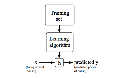
When the target variable that we’re trying to predict is continuous, such as in our housing example, we call the learning problem a regression problem. When y can take on only a small number of discrete values (such as if, given the living area, we wanted to predict if a dwelling is a house or an apartment, say), we call it a classification problem.

4. Cost Function

We can measure the accuracy of our hypothesis function by using a cost function. This takes an average difference (actually a fancier version of an average) of all the results of the hypothesis with inputs from x's and the actual output y's.
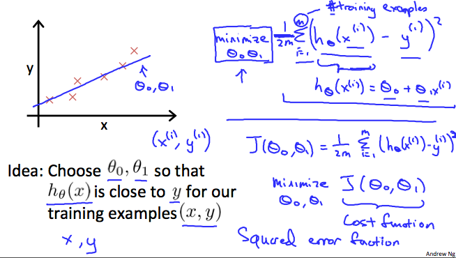
$$
J\left(\theta_{0}, \theta_{1}\right)=\frac{1}{2 m} \sum_{i=1}^{m}\left(\hat{y}{i}-y{i}\right)^{2}=\frac{1}{2 m} \sum_{i=1}^{m}\left(h_{\theta}\left(x_{i}\right)-y_{i}\right)^{2}
$$
To break it apart, it is $\frac{1}{2} \bar{x}$ where $\bar{x}$ is the mean of the squares of $h_\theta (x_{i}) - y_{i}$, or the difference between the predicted value and the actual value.

This function is otherwise called the "Squared error function", or "Mean squared error". The mean is halved $\left(\frac{1}{2}\right)$ as a convenience for the computation of the gradient descent, as the derivative term of the square function will cancel out the $\frac{1}{2}$ term. The following image summarizes what the cost function does:

Cost Function - Intuition I

If we try to think of it in visual terms, our training data set is scattered on the x-y plane. We are trying to make a straight line (defined by $h_\theta(x)$ ) which passes through these scattered data points.

Our objective is to get the best possible line. The best possible line will be such so that the average squared vertical distances of the scattered points from the line will be the least. Ideally, the line should pass through all the points of our training data set. In such a case, the value of $J( \theta_0, \theta_1)$ will be 0. The following example shows the ideal situation where we have a cost function of 0.

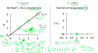
When $\theta_1 = 1$, we get a slope of 1 which goes through every single data point in our model. Conversely, when $\theta_1 = 0.5$ , we see the vertical distance from our fit to the data points increase.

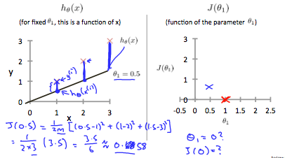
This increases our cost function to 0.58. Plotting several other points yields to the following graph:

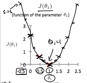
Thus as a goal, we should try to minimize the cost function. In this case, $\theta_1 = 1$ is our global minimum.

Cost Function - Intuition II

A contour plot is a graph that contains many contour lines. A contour line of a two variable function has a constant value at all points of the same line. An example of such a graph is the one to the right below.

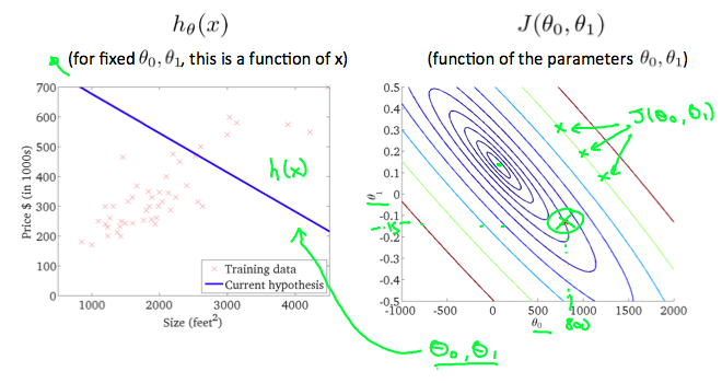
Taking any color and going along the 'circle', one would expect to get the same value of the cost function. For example, the three green points found on the green line above have the same value for $J(\theta_0,\theta_1)$ and as a result, they are found along the same line. The circled x displays the value of the cost function for the graph on the left when $\theta_0 = 800$ and $\theta_1= -0.15$. Taking another h(x) and plotting its contour plot, one gets the following graphs:

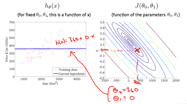
When $\theta_0 = 360$ and $\theta_1 = 0$, the value of $J(\theta_0,\theta_1)$ in the contour plot gets closer to the center thus reducing the cost function error. Now giving our hypothesis function a slightly positive slope results in a better fit of the data.

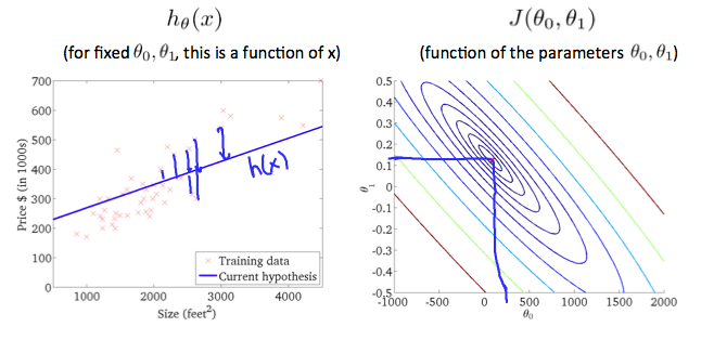
The graph above minimizes the cost function as much as possible and consequently, the result of $\theta_1$ and $\theta_0$ tend to be around 0.12 and 250 respectively. Plotting those values on our graph to the right seems to put our point in the center of the inner most 'circle'.

5. Gradient Descent

So we have our hypothesis function and we have a way of measuring how well it fits into the data. Now we need to estimate the parameters in the hypothesis function. That's where gradient descent comes in.

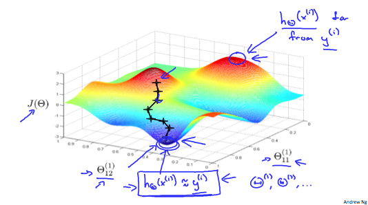
Imagine that we graph our hypothesis function based on its fields $\theta_0$ and $\theta_1$ (actually we are graphing the cost function as a function of the parameter estimates). We are not graphing x and y itself, but the parameter range of our hypothesis function and the cost resulting from selecting a particular set of parameters.

We put $\theta_0$ on the x axis and $\theta_1$ on the y axis, with the cost function on the vertical z axis. The points on our graph will be the result of the cost function using our hypothesis with those specific theta parameters. The graph below depicts such a setup.

We will know that we have succeeded when our cost function is at the very bottom of the pits in our graph, i.e. when its value is the minimum. The red arrows show the minimum points in the graph.

The way we do this is by taking the derivative (the tangential line to a function) of our cost function. The slope of the tangent is the derivative at that point and it will give us a direction to move towards. We make steps down the cost function in the direction with the steepest descent. The size of each step is determined by the parameter α, which is called the learning rate.

For example, the distance between each 'star' in the graph above represents a step determined by our parameter α. A smaller α would result in a smaller step and a larger α results in a larger step. The direction in which the step is taken is determined by the partial derivative of $J(\theta_0,\theta_1)$. Depending on where one starts on the graph, one could end up at different points. The image above shows us two different starting points that end up in two different places.

The gradient descent algorithm is:

repeat until convergence:
$$
\theta_j := \theta_j - \alpha \frac{\partial}{\partial \theta_j} J(\theta_0, \theta_1)
$$
where

j=0,1 represents the feature index number.

At each iteration j, one should simultaneously update the parameters $\theta_1$, $\theta_2$,...,$\theta_n$. Updating a specific parameter prior to calculating another one on the $j^{(th)}$ iteration would yield to a wrong implementation.

1）Gradient Descent Intuition

In this video we explored the scenario where we used one parameter $\theta_1$ and plotted its cost function to implement a gradient descent. Our formula for a single parameter was :

Repeat until convergence:
$$
\theta_1:=\theta_1-\alpha \frac{d}{d\theta_1} J(\theta_1)
$$
Regardless of the slope's sign for $\frac{d}{d\theta_1} J(\theta_1)$, $\theta_1$ eventually converges to its minimum value. The following graph shows that when the slope is negative, the value of $\theta_1$ increases and when it is positive, the value of $\theta_1$ decreases.

On a side note, we should adjust our parameter \alphaα to ensure that the gradient descent algorithm converges in a reasonable time. Failure to converge or too much time to obtain the minimum value imply that our step size is wrong.

How does gradient descent converge with a fixed step size $\alpha$?

The intuition behind the convergence is that $\frac{d}{d\theta_1} J(\theta_1)$ approaches 0 as we approach the bottom of our convex function. At the minimum, the derivative will always be 0 and thus we get:
$$
\theta_1:=\theta_1-\alpha*0
$$

2）Gradient Descent For Linear Regression

Note: [At 6:15 "h(x) = -900 - 0.1x" should be "h(x) = 900 - 0.1x"]

When specifically applied to the case of linear regression, a new form of the gradient descent equation can be derived. We can substitute our actual cost function and our actual hypothesis function and modify the equation to :
$$
\begin{align*} \text{repeat until convergence: } \lbrace & \newline \theta_0 := & \theta_0 - \alpha \frac{1}{m} \sum\limits_{i=1}^{m}(h_\theta(x_{i}) - y_{i}) \newline \theta_1 := & \theta_1 - \alpha \frac{1}{m} \sum\limits_{i=1}^{m}\left((h_\theta(x_{i}) - y_{i}) x_{i}\right) \newline \rbrace& \end{align*}
$$
where m is the size of the training set, $\theta_0$ a constant that will be changing simultaneously with $\theta_1$ and $x_{i}, y_{i}$ are values of the given training set (data).

Note that we have separated out the two cases for $\theta_j$ into separate equations for $\theta_0$ and $\theta_1$; and that for we $\theta_1$ are multiplying $x_{i}$ at the end due to the derivative. The following is a derivation of $\frac {\partial}{\partial \theta_j}J(\theta)$ for a single example :
$$
\begin{aligned}
\frac{\partial}{\partial \theta_{j}} J(\theta) &=\frac{\partial}{\partial \theta_{j}} \frac{1}{2}\left(h_{\theta}(x)-y\right)^{2} \
&=2 \cdot \frac{1}{2}\left(h_{\theta}(x)-y\right) \cdot \frac{\partial}{\partial \theta_{j}}\left(h_{\theta}(x)-y\right) \
&=\left(h_{\theta}(x)-y\right) \cdot \frac{\partial}{\partial \theta_{j}}\left(\sum_{i=0}^{n} \theta_{i} x_{i}-y\right) \
&=\left(h_{\theta}(x)-y\right) x_{j}
\end{aligned}
$$
The point of all this is that if we start with a guess for our hypothesis and then repeatedly apply these gradient descent equations, our hypothesis will become more and more accurate.

So, this is simply gradient descent on the original cost function J. This method looks at every example in the entire training set on every step, and is called batch gradient descent. Note that, while gradient descent can be susceptible to local minima in general, the optimization problem we have posed here for linear regression has only one global, and no other local, optima; thus gradient descent always converges (assuming the learning rate α is not too large) to the global minimum. Indeed, J is a convex quadratic function. Here is an example of gradient descent as it is run to minimize a quadratic function.

The ellipses shown above are the contours of a quadratic function. Also shown is the trajectory taken by gradient descent, which was initialized at (48,30). The x’s in the figure (joined by straight lines) mark the successive values of θ that gradient descent went through as it converged to its minimum.

3）Matrices and Vectors

Matrices are 2-dimensional arrays:
$$
\left[\begin{array}{lllllllll}
a & b & c d & e & f g & h & i j & k & l
\end{array}\right]
$$
The above matrix has four rows and three columns, so it is a 4 x 3 matrix.

A vector is a matrix with one column and many rows:
$$
[w x y z]
$$
So vectors are a subset of matrices. The above vector is a 4 x 1 matrix.

Notation and terms:

• $A_{ij}$ refers to the element in the ith row and jth column of matrix A.
• A vector with 'n' rows is referred to as an 'n'-dimensional vector.
• $v_i$ refers to the element in the ith row of the vector.
• In general, all our vectors and matrices will be 1-indexed. Note that for some programming languages, the arrays are 0-indexed.
• Matrices are usually denoted by uppercase names while vectors are lowercase.
• "Scalar" means that an object is a single value, not a vector or matrix.
• $\mathbb{R}$ refers to the set of scalar real numbers.
• $\mathbb{R^n}$ refers to the set of n-dimensional vectors of real numbers.

Run the cell below to get familiar with the commands in Octave/MATLAB. Feel free to create matrices and vectors and try out different things.

% The ; denotes we are going back to a new row.
A = [1, 2, 3; 4, 5, 6; 7, 8, 9; 10, 11, 12]

% Initialize a vector 
v = [1;2;3] 

% Get the dimension of the matrix A where m = rows and n = columns
[m,n] = size(A)

% You could also store it this way
dim_A = size(A)

% Get the dimension of the vector v 
dim_v = size(v)

% Now let's index into the 2nd row 3rd column of matrix A
A_23 = A(2,3)

Addition and Scalar Multiplication

Addition and subtraction are element-wise, so you simply add or subtract each corresponding element:
$$
\left[\begin{array}{lll}
a & b c & d
\end{array}\right]+\left[\begin{array}{lll}
w & x y & z
\end{array}\right]=\left[\begin{array}{lll}
a+w & b+x c+y & d+z
\end{array}\right]
$$
Subtracting Matrices:
$$
\left[\begin{array}{lll}
a & b c & d
\end{array}\right]-\left[\begin{array}{lll}
w & x y & z
\end{array}\right]=\left[\begin{array}{lll}
a-w & b-x c-y & d-z
\end{array}\right]
$$
To add or subtract two matrices, their dimensions must be the same.

In scalar multiplication, we simply multiply every element by the scalar value:
$$
\left[\begin{array}{lll}
a & b c & d
\end{array}\right]x=\left[\begin{array}{lll}
ax & b * xcx & dx
\end{array}\right]
$$
In scalar division, we simply divide every element by the scalar value:
$$
\left[\begin{array}{lll}
a & b c & d
\end{array}\right]/x=\left[\begin{array}{lll}
/x & b / xc / x & d/x
\end{array}\right]
$$
Experiment below with the Octave/MATLAB commands for matrix addition and scalar multiplication. Feel free to try out different commands. Try to write out your answers for each command before running the cell below.

% Initialize matrix A and B 
A = [1, 2, 4; 5, 3, 2]
B = [1, 3, 4; 1, 1, 1]

% Initialize constant s 
s = 2

% See how element-wise addition works
add_AB = A + B 

% See how element-wise subtraction works
sub_AB = A - B

% See how scalar multiplication works
mult_As = A * s

% Divide A by s
div_As = A / s

% What happens if we have a Matrix + scalar?
add_As = A + s

Matrix-Vector Multiplication

We map the column of the vector onto each row of the matrix, multiplying each element and summing the result.
$$
\left[\begin{array}{llll}
a & b c & \text { de } & f
\end{array}\right] *[x y]=[a * x+b * y c * x+d * y e * x+f * y]
$$
The result is a vector. The number of columns of the matrix must equal the number of rows of the vector.

An m x n matrix multiplied by an n x 1 vector results in an m x 1 vector.

Below is an example of a matrix-vector multiplication. Make sure you understand how the multiplication works. Feel free to try different matrix-vector multiplications.

% Initialize matrix A 
A = [1, 2, 3; 4, 5, 6;7, 8, 9] 

% Initialize vector v 
v = [1; 1; 1] 

% Multiply A * v
Av = A * v

Matrix-Matrix Multiplication

We multiply two matrices by breaking it into several vector multiplications and concatenating the result.
$$
\begin{aligned}
&{\left[\begin{array}{llll}
a & b c & d e & f
\end{array}\right] *\left[\begin{array}{lll}
w & x y & z
\end{array}\right]=} \
&{[a * w+b * y \quad a * x+b * z c * w+d * y \quad c * x+d * z e * w+f * y \quad e * x+f * z]}
\end{aligned}
$$
An m x n matrix multiplied by an n x o matrix results in an m x o matrix. In the above example, a 3 x 2 matrix times a 2 x 2 matrix resulted in a 3 x 2 matrix.

To multiply two matrices, the number of columns of the first matrix must equal the number of rows of the second matrix.

For example:

% Initialize a 3 by 2 matrix 
A = [1, 2; 3, 4;5, 6]

% Initialize a 2 by 1 matrix 
B = [1; 2] 

% We expect a resulting matrix of (3 by 2)*(2 by 1) = (3 by 1) 
mult_AB = A*B

% Make sure you understand why we got that result

Matrix Multiplication Properties

• Matrices are not commutative: $A∗B \neq B∗A$
• Matrices are associative: $(A∗B)∗C = A∗(B∗C)$

The identity matrix, when multiplied by any matrix of the same dimensions, results in the original matrix. It's just like multiplying numbers by 1. The identity matrix simply has 1's on the diagonal (upper left to lower right diagonal) and 0's elsewhere.
$$
\left[\begin{array}{lllllll}
1 & 0 & 00 & 1 & 00 & 0 & 1
\end{array}\right]
$$
When multiplying the identity matrix after some matrix (A∗I), the square identity matrix's dimension should match the other matrix's columns. When multiplying the identity matrix before some other matrix (I∗A), the square identity matrix's dimension should match the other matrix's rows.

% Initialize random matrices A and B 
A = [1,2;4,5]
B = [1,1;0,2]

% Initialize a 2 by 2 identity matrix
I = eye(2)

% The above notation is the same as I = [1,0;0,1]

% What happens when we multiply I*A ? 
IA = I*A 

% How about A*I ? 
AI = A*I 

% Compute A*B 
AB = A*B 

% Is it equal to B*A? 
BA = B*A 

% Note that IA = AI but AB != BA

Inverse and Transpose

The inverse of a matrix $A$ is denoted $A^{-1}$. Multiplying by the inverse results in the identity matrix.

A non square matrix does not have an inverse matrix. We can compute inverses of matrices in octave with the $pinv(A)$ function and in MATLAB with the $inv(A)$ function. Matrices that don't have an inverse are singular or degenerate.

The transposition of a matrix is like rotating the matrix 90° in clockwise direction and then reversing it. We can compute transposition of matrices in MATLAB with the transpose(A) function or A':
$$
A=\left[\begin{array}{llll}
a & b c & d e & f
\end{array}\right]
$$

$$
A^{T}=\left[\begin{array}{lllll}
a & c & e b & d & f
\end{array}\right]
$$

In other words:

$A_{ij} = A^T_{ji}$

% Initialize matrix A 
A = [1,2,0;0,5,6;7,0,9]

% Transpose A 
A_trans = A' 

% Take the inverse of A 
A_inv = inv(A)

% What is A^(-1)*A? 
A_invA = inv(A)*A

Multiple Features

Note: [7:25 - $\theta^T$ is a 1 by (n+1) matrix and not an (n+1) by 1 matrix]

Linear regression with multiple variables is also known as "multivariate linear regression".

We now introduce notation for equations where we can have any number of input variables.
$$
\begin{flalign}
x_j^{(i)}\quad &= \text{value of feature $j$ in the $i^{th}$ training example}&&\
x^{(i)} \quad &= \text{the input (features) of the $i^{th}$ training example}&&\
m \quad &= \text{the number of training examples}&&\
n \quad &= \text{the number of features}&&
\end{flalign}
$$
The multivariable form of the hypothesis function accommodating these multiple features is as follows:
$$
h_\theta(x) = \theta_0+\theta_1x_1+\theta_2x_2+\theta_3x_3+\cdots+\theta_nx_n
$$
In order to develop intuition about this function, we can think about $\theta_0$ as the basic price of a house, $\theta_1$ as the price per square meter, $\theta_2$ as the price per floor, etc. $x_1$ will be the number of square meters in the house, $x_2$ the number of floors, etc.

Using the definition of matrix multiplication, our multivariable hypothesis function can be concisely represented as:
$$
\begin{align*}h_\theta(x) =\begin{bmatrix}\theta_0 \hspace{2em} \theta_1 \hspace{2em} ... \hspace{2em} \theta_n\end{bmatrix}\begin{bmatrix}x_0 \newline x_1 \newline \vdots \newline x_n\end{bmatrix}= \theta^T x\end{align*}
$$
This is a vectorization of our hypothesis function for one training example; see the lessons on vectorization to learn more.

Remark: Note that for convenience reasons in this course we assume $x_{0}^{(i)} =1 \text{ for } (i\in { 1,\dots, m } )$. This allows us to do matrix operations with theta and $x$. Hence making the two vectors '$\theta$' and $x^{(i)}$ match each other element-wise (that is, have the same number of elements: n+1).]

4）Gradient Descent For Multiple Variables

The gradient descent equation itself is generally the same form; we just have to repeat it for our 'n' features:
$$
\begin{align*} & \text{repeat until convergence:} ; \lbrace \newline ; & \theta_0 := \theta_0 - \alpha \frac{1}{m} \sum\limits_{i=1}^{m} (h_\theta(x^{(i)}) - y^{(i)}) \cdot x_0^{(i)}\newline ; & \theta_1 := \theta_1 - \alpha \frac{1}{m} \sum\limits_{i=1}^{m} (h_\theta(x^{(i)}) - y^{(i)}) \cdot x_1^{(i)} \newline ; & \theta_2 := \theta_2 - \alpha \frac{1}{m} \sum\limits_{i=1}^{m} (h_\theta(x^{(i)}) - y^{(i)}) \cdot x_2^{(i)} \newline & \cdots \newline \rbrace \end{align*}
$$
In other words:
$$
\begin{align*}& \text{repeat until convergence:} ; \lbrace \newline ; & \theta_j := \theta_j - \alpha \frac{1}{m} \sum\limits_{i=1}^{m} (h_\theta(x^{(i)}) - y^{(i)}) \cdot x_j^{(i)} ; & \text{for j := 0...n}\newline \rbrace\end{align*}
$$
The following image compares gradient descent with one variable to gradient descent with multiple variables:

5）Gradient Descent in Practice I - Feature Scaling

Note: [6:20 - The average size of a house is 1000 but 100 is accidentally written instead]

We can speed up gradient descent by having each of our input values in roughly the same range. This is because θ will descend quickly on small ranges and slowly on large ranges, and so will oscillate inefficiently down to the optimum when the variables are very uneven.

The way to prevent this is to modify the ranges of our input variables so that they are all roughly the same. Ideally:

−1 ≤ $x_{(i)}$ ≤ 1

or

−0.5 ≤ $x_{(i)}$ ≤ 0.5

These aren't exact requirements; we are only trying to speed things up. The goal is to get all input variables into roughly one of these ranges, give or take a few.

Two techniques to help with this are feature scaling and mean normalization. Feature scaling involves dividing the input values by the range (i.e. the maximum value minus the minimum value) of the input variable, resulting in a new range of just 1. Mean normalization involves subtracting the average value for an input variable from the values for that input variable resulting in a new average value for the input variable of just zero. To implement both of these techniques, adjust your input values as shown in this formula:

$x_i := \dfrac{x_i - \mu_i}{s_i}$

Where $μ_i$ is the average of all the values for feature (i) and $s_i$ is the range of values (max - min), or $s_i$ is the standard deviation.

Note that dividing by the range, or dividing by the standard deviation, give different results. The quizzes in this course use range - the programming exercises use standard deviation.

For example, if $x_i$ represents housing prices with a range of 100 to 2000 and a mean value of 1000, then, $x_i := \dfrac{price-1000}{1900}$

6）Gradient Descent in Practice II - Learning Rate

Note: [5:20 - the x -axis label in the right graph should be \thetaθ rather than No. of iterations ]

Debugging gradient descent. Make a plot with number of iterations on the x-axis. Now plot the cost function, J(θ) over the number of iterations of gradient descent. If J(θ) ever increases, then you probably need to decrease α.

Automatic convergence test. Declare convergence if J(θ) decreases by less than E in one iteration, where E is some small value such as 10^{−3}10−3. However in practice it's difficult to choose this threshold value.

It has been proven that if learning rate α is sufficiently small, then J(θ) will decrease on every iteration.

To summarize:

If $\alpha$ is too small: slow convergence.

If $\alpha$ is too large: may not decrease on every iteration and thus may not converge.

7）Features and Polynomial Regression

We can improve our features and the form of our hypothesis function in a couple different ways.

We can combine multiple features into one. For example, we can combine $x_1$ and $x_2$ into a new feature $x_3$ by taking $x_1⋅x_2$.

Polynomial Regression

Our hypothesis function need not be linear (a straight line) if that does not fit the data well.

We can change the behavior or curve of our hypothesis function by making it a quadratic, cubic or square root function (or any other form).

For example, if our hypothesis function is $h_\theta(x) = \theta_0 + \theta_1 x_1$ then we can create additional features based on $x_1$, to get the quadratic function $h_\theta(x) = \theta_0 + \theta_1 x_1 + \theta_2 x_1^2$ or the cubic function $h_\theta(x) = \theta_0 + \theta_1 x_1 + \theta_2 x_1^2 + \theta_3 x_1^3$

In the cubic version, we have created new features $x_2$ and $x_3$ where $x_2 = x_1^2$ and $x_3 = x_1^3$.

To make it a square root function, we could do: $h_\theta(x) = \theta_0 + \theta_1 x_1 + \theta_2 \sqrt{x_1}$

One important thing to keep in mind is, if you choose your features this way then feature scaling becomes very important.

eg. if $x_1$ has range 1 - 1000 then range of $x_1^2$ becomes 1 - 1000000 and that of $x_1^3$ becomes 1 - 1000000000

6. Computing Parameters Analytically

1) Normal Equation

Note: [8:00 to 8:44 - The design matrix $X$ (in the bottom right side of the slide) given in the example should have elements $x$ with subscript 1 and superscripts varying from 1 to $m$ because for all m training sets there are only 2 features $x_0$ and $x_1$. 12:56 - The $X$ matrix is m by ($n+1$) and NOT $n$ by $n$. ]

Gradient descent gives one way of minimizing $J$. Let’s discuss a second way of doing so, this time performing the minimization explicitly and without resorting to an iterative algorithm. In the "Normal Equation" method, we will minimize $J$ by explicitly taking its derivatives with respect to the $θj$ ’s, and setting them to zero. This allows us to find the optimum theta without iteration. The normal equation formula is given below:
$$
\theta=\left(X^{T} X\right)^{-1} X^{T} y
$$

There is no need to do feature scaling with the normal equation.

The following is a comparison of gradient descent and the normal equation:

Gradient Descent	Normal Equation
Need to choose alpha	No need to choose alpha
Needs many iterations	No need to iterate
$O (kn^2)$	$O (n^3)$, need to calculate inverse of $X^TX$
Works well when $n$ is large	Slow if $n$ is very large

With the normal equation, computing the inversion has complexity $\mathcal{O}(n^3)$. So if we have a very large number of features, the normal equation will be slow. In practice, when n exceeds 10,000 it might be a good time to go from a normal solution to an iterative process.

2) Normal Equation Noninvertibility

When implementing the normal equation in octave we want to use the 'pinv' function rather than 'inv.' The 'pinv' function will give you a value of \thetaθ even if $X^TX$ is not invertible.

If $X^TX$ is noninvertible, the common causes might be having :

• Redundant features, where two features are very closely related (i.e. they are linearly dependent)
• Too many features (e.g. m ≤ n). In this case, delete some features or use "regularization" (to be explained in a later lesson).

Solutions to the above problems include deleting a feature that is linearly dependent with another or deleting one or more features when there are too many features.

7. Classification and Representation

1) Classification

To attempt classification, one method is to use linear regression and map all predictions greater than 0.5 as a 1 and all less than 0.5 as a 0. However, this method doesn't work well because classification is not actually a linear function.

The classification problem is just like the regression problem, except that the values we now want to predict take on only a small number of discrete values. For now, we will focus on the binary classification problem in which y can take on only two values, 0 and 1. (Most of what we say here will also generalize to the multiple-class case.) For instance, if we are trying to build a spam classifier for email, then $x^{(i)}$ may be some features of a piece of email, and y may be 1 if it is a piece of spam mail, and 0 otherwise. Hence, y∈{0, 1}. 0 is also called the negative class, and 1 the positive class, and they are sometimes also denoted by the symbols “-” and “+.” Given $x^{(i)}$ , the corresponding $y^{(i)}$ is also called the label for the training example.

2) Hypothesis Representation

We could approach the classification problem ignoring the fact that y is discrete-valued, and use our old linear regression algorithm to try to predict y given x. However, it is easy to construct examples where this method performs very poorly. Intuitively, it also doesn’t make sense for $h_\theta (x)$ to take values larger than 1 or smaller than 0 when we know that $y ∈ {0, 1}$. To fix this, let’s change the form for our hypotheses $h_\theta (x)$ to satisfy $0 \leq h_\theta (x) \leq 1$. This is accomplished by plugging $\theta^Tx$ into the Logistic Function.

Our new form uses the "Sigmoid Function," also called the "Logistic Function":
$$
\begin{align*}& h_\theta (x) = g ( \theta^T x ) \newline \newline& z = \theta^T x \newline& g(z) = \dfrac{1}{1 + e^{-z}}\end{align*}
$$
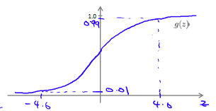
The following image shows us what the sigmoid function looks like:

The function $g(z)$, shown here, maps any real number to the $(0, 1)$ interval, making it useful for transforming an arbitrary-valued function into a function better suited for classification.

$h_\theta(x)$ will give us the probability that our output is 1. For example, $h_\theta(x)=0.7$ gives us a probability of 70% that our output is 1. Our probability that our prediction is 0 is just the complement of our probability that it is 1 (e.g. if probability that it is 1 is 70%, then the probability that it is 0 is 30%).
$$
\begin{align*}& h_\theta(x) = P(y=1 | x ; \theta) = 1 - P(y=0 | x ; \theta) \newline& P(y = 0 | x;\theta) + P(y = 1 | x ; \theta) = 1\end{align*}
$$

3) Decision Boundary

In order to get our discrete 0 or 1 classification, we can translate the output of the hypothesis function as follows:
$$
\begin{align*}& h_\theta(x) \geq 0.5 \rightarrow y = 1 \newline& h_\theta(x) < 0.5 \rightarrow y = 0 \newline\end{align*}
$$
The way our logistic function g behaves is that when its input is greater than or equal to zero, its output is greater than or equal to 0.5:
$$
\begin{align*}& g(z) \geq 0.5 \newline& when ; z \geq 0\end{align*}
$$
Remember.
$$
\begin{align*}z=0, e^{0}=1 \Rightarrow g(z)=1/2\newline z \to \infty, e^{-\infty} \to 0 \Rightarrow g(z)=1 \newline z \to -\infty, e^{\infty}\to \infty \Rightarrow g(z)=0 \end{align*}
$$
So if our input to g $is \theta^T X$, then that means:
$$
\begin{align*}& h_\theta(x) = g(\theta^T x) \geq 0.5 \newline& when ; \theta^T x \geq 0\end{align*}
$$
From these statements we can now say:
$$
\begin{align*}& \theta^T x \geq 0 \Rightarrow y = 1 \newline& \theta^T x < 0 \Rightarrow y = 0 \newline\end{align*}
$$
The decision boundary is the line that separates the area where y = 0 and where y = 1. It is created by our hypothesis function.

Example:
$$
\begin{align*}& \theta = \begin{bmatrix}5 \newline -1 \newline 0\end{bmatrix} \newline & y = 1 ; if ; 5 + (-1) x_1 + 0 x_2 \geq 0 \newline & 5 - x_1 \geq 0 \newline & - x_1 \geq -5 \newline& x_1 \leq 5 \newline \end{align*}
$$
In this case, our decision boundary is a straight vertical line placed on the graph where $x_1$ = 5, and everything to the left of that denotes $y = 1$, while everything to the right denotes $y = 0$.

Again, the input to the sigmoid function $g(z)$ (e.g. $\theta^T X$) doesn't need to be linear, and could be a function that describes a circle (e.g. $z = \theta_0 + \theta_1 x_1^2 +\theta_2 x_2^2$) or any shape to fit our data.

4) Cost Function

We cannot use the same cost function that we use for linear regression because the Logistic Function will cause the output to be wavy, causing many local optima. In other words, it will not be a convex function.

Instead, our cost function for logistic regression looks like:
$$
\begin{align*}& J(\theta) = \dfrac{1}{m} \sum_{i=1}^m \mathrm{Cost}(h_\theta(x^{(i)}),y^{(i)}) \newline & \mathrm{Cost}(h_\theta(x),y) = -\log(h_\theta(x)) ; & \text{if y = 1} \newline & \mathrm{Cost}(h_\theta(x),y) = -\log(1-h_\theta(x)) ; & \text{if y = 0}\end{align*}
$$
When $y = 1$, we get the following plot for $J(\theta)$ vs $h_\theta (x)$:

Similarly, when $y = 0$, we get the following plot for $ J(\theta)$ vs $h_\theta (x)$:

$$
\begin{align*}& \mathrm{Cost}(h_\theta(x),y) = 0 \text{ if } h_\theta(x) = y \newline & \mathrm{Cost}(h_\theta(x),y) \rightarrow \infty \text{ if } y = 0 ; \mathrm{and} ; h_\theta(x) \rightarrow 1 \newline & \mathrm{Cost}(h_\theta(x),y) \rightarrow \infty \text{ if } y = 1 ; \mathrm{and} ; h_\theta(x) \rightarrow 0 \newline \end{align*}
$$
If our correct answer 'y' is 0, then the cost function will be 0 if our hypothesis function also outputs 0. If our hypothesis approaches 1, then the cost function will approach infinity.

If our correct answer 'y' is 1, then the cost function will be 0 if our hypothesis function outputs 1. If our hypothesis approaches 0, then the cost function will approach infinity.

Note that writing the cost function in this way guarantees that $J(\theta)$ is convex for logistic regression.

5) Simplified Cost Function and Gradient Descent

Note: [6:53 - the gradient descent equation should have a 1/m factor]

We can compress our cost function's two conditional cases into one case:
$$
\operatorname{Cost}\left(h_{\theta}(x), y\right)=-y \log \left(h_{\theta}(x)\right)-(1-y) \log \left(1-h_{\theta}(x)\right)
$$
Notice that when y is equal to 1, then the second term $(1-y)\log(1-h_\theta(x))$ will be zero and will not affect the result. If y is equal to 0, then the first term $-y \log(h_\theta(x))$ will be zero and will not affect the result.

We can fully write out our entire cost function as follows:
$$
J(\theta)=-\frac{1}{m} \sum_{i=1}^{m}\left[y^{(i)} \log \left(h_{\theta}\left(x^{(i)}\right)\right)+\left(1-y^{(i)}\right) \log \left(1-h_{\theta}\left(x^{(i)}\right)\right)\right]
$$
A vectorized implementation is:
$$
\begin{align*} & h = g(X\theta)\newline & J(\theta) = \frac{1}{m} \cdot \left(-y^{T}\log(h)-(1-y)^{T}\log(1-h)\right) \end{align*}
$$

Gradient Descent

Remember that the general form of gradient descent is:
$$
\begin{align*} & Repeat ; \lbrace \newline & ; \theta_j := \theta_j - \frac{\alpha}{m} \sum_{i=1}^m (h_\theta(x^{(i)}) - y^{(i)}) x_j^{(i)} \newline & \rbrace \end{align*}
$$
Notice that this algorithm is identical to the one we used in linear regression. We still have to simultaneously update all values in theta.

A vectorized implementation is:
$$
\theta:=\theta-\frac{\alpha}{m} X^{T}(g(X \theta)-\vec{y})
$$

6) Advanced Optimization

Note: [7:35 - '100' should be 100 instead. The value provided should be an integer and not a character string.]

"Conjugate gradient", "BFGS", and "L-BFGS" are more sophisticated, faster ways to optimize θ that can be used instead of gradient descent. We suggest that you should not write these more sophisticated algorithms yourself (unless you are an expert in numerical computing) but use the libraries instead, as they're already tested and highly optimized. Octave provides them.

We first need to provide a function that evaluates the following two functions for a given input value $θ$:
$$
\begin{aligned}
&J(\theta) \
&\frac{\partial}{\partial \theta_{j}} J(\theta)
\end{aligned}
$$
We can write a single function that returns both of these:

function [jVal, gradient] = costFunction(theta)
    jVal = [...code to compute J(theta)...];
  gradient = [...code to compute derivative of J(theta)...];
end

Then we can use octave's "fminunc()" optimization algorithm along with the "optimset()" function that creates an object containing the options we want to send to "fminunc()". (Note: the value for MaxIter should be an integer, not a character string - errata in the video at 7:30)

options = optimset('GradObj', 'on', 'MaxIter', 100);
initialTheta = zeros(2,1);
   [optTheta, functionVal, exitFlag] = fminunc(@costFunction, initialTheta, options);

We give to the function ‘fminunc()’ our cost function, our initial vector of theta values, and the "options" object that we created beforehand.

7) Multiclass Classification: One-vs-all

Now we will approach the classification of data when we have more than two categories. Instead of $y = {0,1}$ we will expand our definition so that $y = {0,1...n}$.

Since $y = {0,1...n}$, we divide our problem into $n+1$ ($+1$ because the index starts at $0$) binary classification problems; in each one, we predict the probability that 'y' is a member of one of our classes.
$$
\begin{align*}& y \in \lbrace0, 1 ... n\rbrace \newline& h_\theta^{(0)}(x) = P(y = 0 | x ; \theta) \newline& h_\theta^{(1)}(x) = P(y = 1 | x ; \theta) \newline& \cdots \newline& h_\theta^{(n)}(x) = P(y = n | x ; \theta) \newline& \mathrm{prediction} = \max_i( h_\theta ^{(i)}(x) )\newline\end{align*}
$$
We are basically choosing one class and then lumping all the others into a single second class. We do this repeatedly, applying binary logistic regression to each case, and then use the hypothesis that returned the highest value as our prediction.

The following image shows how one could classify 3 classes:

To summarize:

Train a logistic regression classifier $h_\theta^{(i)}(x)$ for each class $i$ to predict the probability that $y = i$

To make a prediction on a new $x$, pick the class $i$ that maximizes $\max \left{h_{\theta}^{(i)}(x)\right}$

8. Solving the Problem of Overfitting

The Problem of Overfitting

Consider the problem of predicting $y$ from $x ∈ R$. The leftmost figure below shows the result of fitting a $y = θ_0 + θ_1x$ to a dataset. We see that the data doesn’t really lie on straight line, and so the fit is not very good.

Instead, if we had added an extra feature $x^2$ , and fit $y = \theta_0 + \theta_1x + \theta_2x^2$ , then we obtain a slightly better fit to the data (See middle figure). Naively, it might seem that the more features we add, the better. However, there is also a danger in adding too many features: The rightmost figure is the result of fitting a $5^{th}$ order polynomial $y = \sum_{j=0} ^5 \theta_j x^j$. We see that even though the fitted curve passes through the data perfectly, we would not expect this to be a very good predictor of, say, housing prices ($y$) for different living areas ($x$). Without formally defining what these terms mean, we’ll say the figure on the left shows an instance of underfitting—in which the data clearly shows structure not captured by the model—and the figure on the right is an example of overfitting.

Underfitting, or high bias, is when the form of our hypothesis function h maps poorly to the trend of the data. It is usually caused by a function that is too simple or uses too few features. At the other extreme, overfitting, or high variance, is caused by a hypothesis function that fits the available data but does not generalize well to predict new data. It is usually caused by a complicated function that creates a lot of unnecessary curves and angles unrelated to the data.

This terminology is applied to both linear and logistic regression. There are two main options to address the issue of overfitting:

1. Reduce the number of features:

• Manually select which features to keep.
• Use a model selection algorithm (studied later in the course).

2. Regularization

• Keep all the features, but reduce the magnitude of parameters $\theta_j$.
• Regularization works well when we have a lot of slightly useful features.

Cost Function

Note: [5:18 - There is a typo. It should be $\sum_{j=1}^{n} \theta j ^2$ instead of $\sum{i=1}^{n} \theta _j ^2$]

If we have overfitting from our hypothesis function, we can reduce the weight that some of the terms in our function carry by increasing their cost.

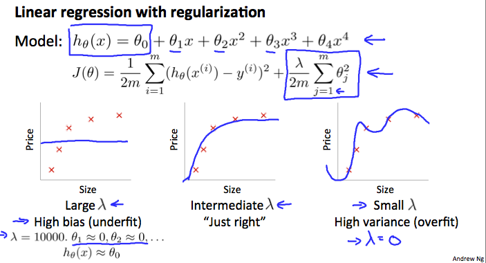
Say we wanted to make the following function more quadratic:
$$
\theta_{0}+\theta_{1} x +\theta_{2} x^{2}+\theta_{3} x^{3}+\theta_{4} x^{4}
$$
We'll want to eliminate the influence of$ \theta_3x^3$ and $\theta_4x^4$ . Without actually getting rid of these features or changing the form of our hypothesis, we can instead modify our cost function:
$$
\min {\theta} \frac{1}{2 m} \sum{i=1}^{m}\left(h_{\theta}\left(x^{(i)}\right)-y^{(i)}\right)^{2}+1000 \cdot \theta_{3}^{2}+1000 \cdot \theta_{4}^{2}
$$
We've added two extra terms at the end to inflate the cost of and $\theta_4$. Now, in order for the cost function to get close to zero, we will have to reduce the values of $\theta_3$ and $\theta_4$ to near zero. This will in turn greatly reduce the values of $\theta_3x^3$ and $\theta_4x^4$ in our hypothesis function. As a result, we see that the new hypothesis (depicted by the pink curve) looks like a quadratic function but fits the data better due to the extra small terms $\theta_3x^3$ and $\theta_4x^4$.

We could also regularize all of our theta parameters in a single summation as:
$$
\min {\theta} \frac{1}{2 m} \left(\sum{i=1}^{m}\left(h_{\theta}\left(x^{(i)}\right)-y^{(i)}\right)^{2}+\lambda \sum_{j=1}^{n} \theta_{j}^{2}\right)
$$
The λ, or lambda, is the regularization parameter. It determines how much the costs of our theta parameters are inflated.

Using the above cost function with the extra summation, we can smooth the output of our hypothesis function to reduce overfitting. If lambda is chosen to be too large, it may smooth out the function too much and cause underfitting. Hence, what would happen if $\lambda = 0$ or is too small ?

Regularized Linear Regression

Note: [8:43 - It is said that X is non-invertible if m $\leq$ n. The correct statement should be that X is non-invertible if m < n, and may be non-invertible if m = n.

We can apply regularization to both linear regression and logistic regression. We will approach linear regression first.

Gradient Descent

We will modify our gradient descent function to separate out $\theta_0$ from the rest of the parameters because we do not want to penalize $\theta_0$.

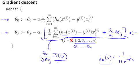
$$
\begin{align*} & \text{Repeat}\ \lbrace \newline & \ \ \ \ \theta_0 := \theta_0 - \alpha\ \frac{1}{m}\ \sum_{i=1}^m (h_\theta(x^{(i)}) - y^{(i)})x_0^{(i)} \newline & \ \ \ \ \theta_j := \theta_j - \alpha\ \left[ \left( \frac{1}{m}\ \sum_{i=1}^m (h_\theta(x^{(i)}) - y^{(i)})x_j^{(i)} \right) + \frac{\lambda}{m}\theta_j \right] &\ \ \ \ \ \ \ \ \ \ j \in \lbrace 1,2...n\rbrace\newline & \rbrace \end{align*}
$$

The term $\frac{\lambda}{m}\theta_j$ performs our regularization. With some manipulation our update rule can also be represented as:

$$
\theta_{j}:=\theta_{j}\left(1-\alpha \frac{\lambda}{m}\right)-\alpha \frac{1}{m} \sum_{i=1}^{m}\left(h_{\theta}\left(x^{(i)}\right)-y^{(i)}\right) x_{j}^{(i)}
$$

The first term in the above equation, $1 - \alpha\frac{\lambda}{m}$ will always be less than 1. Intuitively you can see it as reducing the value of $\theta_j$ by some amount on every update. Notice that the second term is now exactly the same as it was before.

Normal Equation

Now let's approach regularization using the alternate method of the non-iterative normal equation.

To add in regularization, the equation is the same as our original, except that we add another term inside the parentheses:
$$
\begin{align*}& \theta = \left( X^TX + \lambda \cdot L \right)^{-1} X^Ty \newline& \text{where}\ \ L = \begin{bmatrix} 0 & & & & \newline & 1 & & & \newline & & 1 & & \newline & & & \ddots & \newline & & & & 1 \newline\end{bmatrix}\end{align*}
$$
L is a matrix with 0 at the top left and 1's down the diagonal, with 0's everywhere else. It should have dimension $(n+1)×(n+1)$. Intuitively, this is the identity matrix (though we are not including x_0x0), multiplied with a single real number λ.

Recall that if m < n, then $X^TX$ is non-invertible. However, when we add the term $λ⋅L$, then $X^TX + λ⋅L$ becomes invertible.

Regularized Logistic Regression

We can regularize logistic regression in a similar way that we regularize linear regression. As a result, we can avoid overfitting. The following image shows how the regularized function, displayed by the pink line, is less likely to overfit than the non-regularized function represented by the blue line:

Cost Function

Recall that our cost function for logistic regression was:

$$
J(\theta)=-\frac{1}{m} \sum_{i=1}^{m}\left[y^{(i)} \log \left(h_{\theta}\left(x^{(i)}\right)\right)+\left(1-y^{(i)}\right) \log \left(1-h_{\theta}\left(x^{(i)}\right)\right)\right]
$$
We can regularize this equation by adding a term to the end:

$$
J(\theta)=-\frac{1}{m} \sum_{i=1}^{m}\left[y^{(i)} \log \left(h_{\theta}\left(x^{(i)}\right)\right)+\left(1-y^{(i)}\right) \log \left(1-h_{\theta}\left(x^{(i)}\right)\right)\right]+\frac{\lambda}{2 m} \sum_{j=1}^{n} \theta_{j}^{2}
$$

The second sum, $\sum_{j=1}^n \theta_j^2$ means to explicitly exclude the bias term, $\theta_0$. I.e. the $θ$ vector is indexed from $0$ to $n$ (holding $n+1$ values, \theta_0 through $\theta_n$), and this sum explicitly skips $\theta_0$, by running from $1$ to $n$, skipping $0$. Thus, when computing the equation, we should continuously update the two following equations:

9. Neural Networks: Representation

Neural Networks

Model Representation I

Let's examine how we will represent a hypothesis function using neural networks. At a very simple level, neurons are basically computational units that take inputs (dendrites) as electrical inputs (called "spikes") that are channeled to outputs (axons). In our model, our dendrites are like the input features $x_1\cdots x_n$, and the output is the result of our hypothesis function. In this model our $x_0$x0​ input node is sometimes called the "bias unit." It is always equal to 1. In neural networks, we use the same logistic function as in classification, $\frac{1}{1 + e^{-\theta^Tx}}$, yet we sometimes call it a sigmoid (logistic) activation function. In this situation, our "theta" parameters are sometimes called "weights".

Visually, a simplistic representation looks like:

$$
\left[x_{0} x_{1} x_{2}\right] \rightarrow[\quad] \rightarrow h_{\theta}(x)
$$

Our input nodes (layer 1), also known as the "input layer", go into another node (layer 2), which finally outputs the hypothesis function, known as the "output layer".

We can have intermediate layers of nodes between the input and output layers called the "hidden layers."

In this example, we label these intermediate or "hidden" layer nodes $a^2_0 \cdots a^2_n$ and call them "activation units."

$$
\begin{align*}& a_i^{(j)} = \text{"activation" of unit $i$ in layer $j$} \newline& \Theta^{(j)} = \text{matrix of weights controlling function mapping from layer $j$ to layer $j+1$}\end{align*}
$$

If we had one hidden layer, it would look like:

$$
\left[x_{0} x_{1} x_{2} x_{3}\right] \rightarrow\left[a_{1}^{(2)} a_{2}^{(2)} a_{3}^{(2)}\right] \rightarrow h_{\theta}(x)
$$

The values for each of the "activation" nodes is obtained as follows:

$$
\begin{align*} a_1^{(2)} = g(\Theta_{10}^{(1)}x_0 + \Theta_{11}^{(1)}x_1 + \Theta_{12}^{(1)}x_2 + \Theta_{13}^{(1)}x_3) \newline a_2^{(2)} = g(\Theta_{20}^{(1)}x_0 + \Theta_{21}^{(1)}x_1 + \Theta_{22}^{(1)}x_2 + \Theta_{23}^{(1)}x_3) \newline a_3^{(2)} = g(\Theta_{30}^{(1)}x_0 + \Theta_{31}^{(1)}x_1 + \Theta_{32}^{(1)}x_2 + \Theta_{33}^{(1)}x_3) \newline h_\Theta(x) = a_1^{(3)} = g(\Theta_{10}^{(2)}a_0^{(2)} + \Theta_{11}^{(2)}a_1^{(2)} + \Theta_{12}^{(2)}a_2^{(2)} + \Theta_{13}^{(2)}a_3^{(2)}) \newline \end{align*}
$$

This is saying that we compute our activation nodes by using a 3×4 matrix of parameters. We apply each row of the parameters to our inputs to obtain the value for one activation node. Our hypothesis output is the logistic function applied to the sum of the values of our activation nodes, which have been multiplied by yet another parameter matrix $\Theta^{(2)}$ containing the weights for our second layer of nodes.

Each layer gets its own matrix of weights, $\Theta^{(j)}$.

The dimensions of these matrices of weights is determined as follows:

$$
\text{If network has $s_j$ units in layer $j$ and $s_{j+1}$ units in layer $j+1$, then $\Theta^{(j)}$ will be of dimension $s_{j+1} \times (s_j + 1)$.}
$$

The +1 comes from the addition in $\Theta^{(j)}$ of the "bias nodes," $x_0$ and $\Theta_0^{(j)}$. In other words the output nodes will not include the bias nodes while the inputs will. The following image summarizes our model representation:

Example: If layer 1 has 2 input nodes and layer 2 has 4 activation nodes. Dimension of $\Theta^{(1)}$ is going to be 4×3 where $s_j = 2$ and $s_{j+1} = 4$, so $s_{j+1} \times (s_j + 1) = 4 \times 3$.

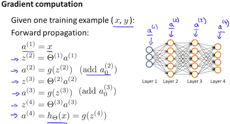
Model Representation II

To re-iterate, the following is an example of a neural network:

$$
\begin{align*} a_1^{(2)} = g(\Theta_{10}^{(1)}x_0 + \Theta_{11}^{(1)}x_1 + \Theta_{12}^{(1)}x_2 + \Theta_{13}^{(1)}x_3) \newline a_2^{(2)} = g(\Theta_{20}^{(1)}x_0 + \Theta_{21}^{(1)}x_1 + \Theta_{22}^{(1)}x_2 + \Theta_{23}^{(1)}x_3) \newline a_3^{(2)} = g(\Theta_{30}^{(1)}x_0 + \Theta_{31}^{(1)}x_1 + \Theta_{32}^{(1)}x_2 + \Theta_{33}^{(1)}x_3) \newline h_\Theta(x) = a_1^{(3)} = g(\Theta_{10}^{(2)}a_0^{(2)} + \Theta_{11}^{(2)}a_1^{(2)} + \Theta_{12}^{(2)}a_2^{(2)} + \Theta_{13}^{(2)}a_3^{(2)}) \newline \end{align*}
$$

In this section we'll do a vectorized implementation of the above functions. We're going to define a new variable $z_k^{(j)}$ that encompasses the parameters inside our g function. In our previous example if we replaced by the variable z for all the parameters we would get:

$$
\begin{align*}a_1^{(2)} = g(z_1^{(2)}) \newline a_2^{(2)} = g(z_2^{(2)}) \newline a_3^{(2)} = g(z_3^{(2)}) \newline \end{align*}
$$

In other words, for layer j=2 and node k, the variable z will be:

$$
z_{k}^{(2)}=\Theta_{k, 0}^{(1)} x_{0}+\Theta_{k, 1}^{(1)} x_{1}+\cdots+\Theta_{k, n}^{(1)} x_{n}
$$

The vector representation of x and $z^{j}$ is:

$$
\begin{align*}x = \begin{bmatrix}x_0 \newline x_1 \newline\cdots \newline x_n\end{bmatrix} &z^{(j)} = \begin{bmatrix}z_1^{(j)} \newline z_2^{(j)} \newline\cdots \newline z_n^{(j)}\end{bmatrix}\end{align*}
$$

Setting $x = a^{(1)}$, we can rewrite the equation as:

$$
z^{(j)}=\Theta^{(j-1)} a^{(j-1)}
$$

We are multiplying our matrix $\Theta^{(j-1)}$ with dimensions $s_j\times (n+1)$ (where $s_j$ is the number of our activation nodes) by our vector$ a^{(j-1)}$ with height $(n+1)$. This gives us our vector$ z^{(j)}$ with height $s_j$. Now we can get a vector of our activation nodes for layer j as follows:

$a^{(j)} = g(z^{(j)})$

Where our function g can be applied element-wise to our vector $z^{(j)}$.

We can then add a bias unit (equal to 1) to layer j after we have computed $a^{(j)}$. This will be element $a_0^{(j)}$ and will be equal to 1. To compute our final hypothesis, let's first compute another z vector:

$z^{(j+1)} = \Theta^{(j)}a^{(j)}$

We get this final z vector by multiplying the next theta matrix after $\Theta^{(j-1)}$ with the values of all the activation nodes we just got. This last theta matrix $\Theta^{(j)}$ will have only one row which is multiplied by one column $a^{(j)}$ so that our result is a single number. We then get our final result with:

$h_\Theta(x) = a^{(j+1)} = g(z^{(j+1)})$

Notice that in this last step, between layer j and layer j+1, we are doing exactly the same thing as we did in logistic regression. Adding all these intermediate layers in neural networks allows us to more elegantly produce interesting and more complex non-linear hypotheses.

Examples and Intuitions I

A simple example of applying neural networks is by predicting $x_1$ AND $x_2$, which is the logical 'and' operator and is only true if both $x_1$ and $x_2$ are 1.

The graph of our functions will look like:

$$
\begin{align*}\begin{bmatrix}x_0 \newline x_1 \newline x_2\end{bmatrix} \rightarrow\begin{bmatrix}g(z^{(2)})\end{bmatrix} \rightarrow h_\Theta(x)\end{align*}
$$

Remember that $x_0$ is our bias variable and is always 1.

Let's set our first theta matrix as:

$$
\Theta^{(2)}=\left[\begin{array}{lll}
-30 & 20 & 20
\end{array}\right]
$$

This will cause the output of our hypothesis to only be positive if both $x_1$ and $x_2$ are $1$. In other words:

$$
\begin{align*}& h_\Theta(x) = g(-30 + 20x_1 + 20x_2) \newline \newline & x_1 = 0 \ \ and \ \ x_2 = 0 \ \ then \ \ g(-30) \approx 0 \newline & x_1 = 0 \ \ and \ \ x_2 = 1 \ \ then \ \ g(-10) \approx 0 \newline & x_1 = 1 \ \ and \ \ x_2 = 0 \ \ then \ \ g(-10) \approx 0 \newline & x_1 = 1 \ \ and \ \ x_2 = 1 \ \ then \ \ g(10) \approx 1\end{align*}
$$

So we have constructed one of the fundamental operations in computers by using a small neural network rather than using an actual AND gate. Neural networks can also be used to simulate all the other logical gates. The following is an example of the logical operator 'OR', meaning either $x_1$ is true or $x_2$ is true, or both:

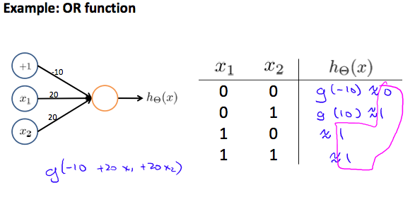
Where g(z) is the following:

Examples and Intuitions II

The $Θ^{(1)}$ matrices for AND, NOR, and OR are:

$$
\begin{align*}AND:\newline\Theta^{(1)} &=\begin{bmatrix}-30 & 20 & 20\end{bmatrix} \newline NOR:\newline\Theta^{(1)} &= \begin{bmatrix}10 & -20 & -20\end{bmatrix} \newline OR:\newline\Theta^{(1)} &= \begin{bmatrix}-10 & 20 & 20\end{bmatrix} \newline\end{align*}
$$

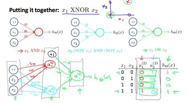
We can combine these to get the XNOR logical operator (which gives 1 $if x_1$ and $x_2$ are both 0 or both 1).

$$
\begin{align*}\begin{bmatrix}x_0 \newline x_1 \newline x_2\end{bmatrix} \rightarrow\begin{bmatrix}a_1^{(2)} \newline a_2^{(2)} \end{bmatrix} \rightarrow\begin{bmatrix}a^{(3)}\end{bmatrix} \rightarrow h_\Theta(x)\end{align*}
$$
For the transition between the first and second layer, we'll use a $Θ^{(1)}$ matrix that combines the values for AND and NOR:
$$
\Theta^{(1)}=\left[\begin{array}{lll}
-30 & 20 & 2010 & -20 & -20
\end{array}\right]
$$
For the transition between the second and third layer, we'll use a $Θ^{(2)}$ matrix that uses the value for OR:

$$
\Theta^{(2)}=\left[\begin{array}{lll}
-10 & 20 & 20
\end{array}\right]
$$
Let's write out the values for all our nodes:
$$
\begin{align*}& a^{(2)} = g(\Theta^{(1)} \cdot x) \newline& a^{(3)} = g(\Theta^{(2)} \cdot a^{(2)}) \newline& h_\Theta(x) = a^{(3)}\end{align*}
$$
And there we have the XNOR operator using a hidden layer with two nodes! The following summarizes the above algorithm:

Multiclass Classification

To classify data into multiple classes, we let our hypothesis function return a vector of values. Say we wanted to classify our data into one of four categories. We will use the following example to see how this classification is done. This algorithm takes as input an image and classifies it accordingly:

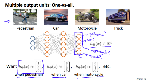
We can define our set of resulting classes as y:

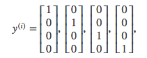
Each $y^{(i)}y (i)$ represents a different image corresponding to either a car, pedestrian, truck, or motorcycle. The inner layers, each provide us with some new information which leads to our final hypothesis function. The setup looks like:

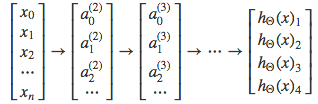
Our resulting hypothesis for one set of inputs may look like:
$$
h_{\theta} = \begin{bmatrix}0 \newline 0 \newline 1 \newline 0\end{bmatrix}
$$
In which case our resulting class is the third one down, or $h_\Theta(x)_3$, which represents the motorcycle.

10. Neural Networks: Learning

1) Cost Function and Backpropagation

Cost Function

Let's first define a few variables that we will need to use:

• L = total number of layers in the network

• $s_l$ = number of units (not counting bias unit) in layer l

• K = number of output units/classes

Recall that in neural networks, we may have many output nodes. We denote $h_\Theta(x)k$ as being a hypothesis that results in the $k^{th}$ output. Our cost function for neural networks is going to be a generalization of the one we used for logistic regression. Recall that the cost function for regularized logistic regression was:
$$
J(\theta)=-\frac{1}{m} \sum{i=1}^{m}\left[y^{(i)} \log \left(h_{\theta}\left(x^{(i)}\right)\right)+\left(1-y^{(i)}\right) \log \left(1-h_{\theta}\left(x^{(i)}\right)\right)\right]+\frac{\lambda}{2 m} \sum_{j=1}^{n} \theta_{j}^{2}
$$
For neural networks, it is going to be slightly more complicated:
$$
J(\Theta)=-\frac{1}{m} \sum_{i=1}^{m} \sum_{k=1}^{K}\left[y_{k}^{(i)} \log \left(\left(h_{\Theta}\left(x^{(i)}\right)\right){k}\right)+\left(1-y{k}^{(i)}\right) \log \left(1-\left(h_{\Theta}\left(x^{(i)}\right)\right){k}\right)\right]+\frac{\lambda}{2 m} \sum{l=1}^{L-1} \sum_{i=1}^{s_{l}} \sum_{j=1}^{s_{l+1}}\left(\Theta_{j, i}^{(l)}\right)^{2}
$$
We have added a few nested summations to account for our multiple output nodes. In the first part of the equation, before the square brackets, we have an additional nested summation that loops through the number of output nodes.

In the regularization part, after the square brackets, we must account for multiple theta matrices. The number of columns in our current theta matrix is equal to the number of nodes in our current layer (including the bias unit). The number of rows in our current theta matrix is equal to the number of nodes in the next layer (excluding the bias unit). As before with logistic regression, we square every term.

Note:

• the double sum simply adds up the logistic regression costs calculated for each cell in the output layer

• the triple sum simply adds up the squares of all the individual Θs in the entire network.

• the i in the triple sum does not refer to training example i

Backpropagation Algorithm

"Backpropagation" is neural-network terminology for minimizing our cost function, just like what we were doing with gradient descent in logistic and linear regression. Our goal is to compute:
$$min_{\Theta} J(\Theta)$$

That is, we want to minimize our cost function J using an optimal set of parameters in theta. In this section we'll look at the equations we use to compute the partial derivative of J(Θ):
$$
\frac{\partial}{\partial \Theta_{i, j}^{(l)}} J(\Theta)
$$
To do so, we use the following algorithm:

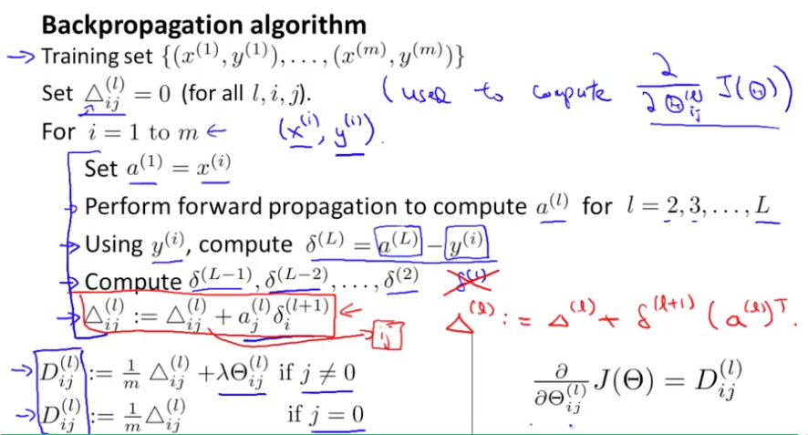
Back propagation Algorithm

Given training set $\lbrace (x^{(1)}, y^{(1)}) \cdots (x^{(m)}, y^{(m)})\rbrace{(x(1),y(1))⋯(x(m),y(m))}$

• Set $\Delta^{(l)}_{i,j}Δi,j(l)​ := 0 \quad \text{for all (l,i,j)}$, (hence you end up having a matrix full of zeros)

For training example t =1 to m:

1. Set $a^{(1)} := x^{(t)}$

2. Perform forward propagation to compute $a^{(l)}$ for $l=2,3,…,L$

3. Using $y^{(t)}$, compute $\delta^{(L)} = a^{(L)} - y^{(t)}$

Where L is our total number of layers and a^{(L)}a(L) is the vector of outputs of the activation units for the last layer. So our "error values" for the last layer are simply the differences of our actual results in the last layer and the correct outputs in y. To get the delta values of the layers before the last layer, we can use an equation that steps us back from right to left:

4. Compute $\delta^{(L-1)}, \delta^{(L-2)},\dots,\delta^{(2)}δ(L−1),δ(L−2),…,δ(2)$ using $\delta^{(l)} = ((\Theta^{(l)})^T \delta^{(l+1)})\ .*\ a^{(l)}\ .*\ (1 - a^{(l)})$

The delta values of layer l are calculated by multiplying the delta values in the next layer with the theta matrix of layer l. We then element-wise multiply that with a function called g', or g-prime, which is the derivative of the activation function g evaluated with the input values given by $z^{(l)}$.

The g-prime derivative terms can also be written out as:
$$
g^{\prime}\left(z^{(l)}\right)=a^{(l)} \cdot *\left(1-a^{(l)}\right)
$$
5. $\Delta^{(l)}{i,j} := \Delta^{(l)}{i,j} + a_j^{(l)} \delta_i^{(l+1)}$ or with vectorization, $\Delta^{(l)} := \Delta^{(l)} + \delta^{(l+1)}(a^{(l)})^T$

Hence we update our new $\Delta$ matrix.

• $D^{(l)}{i,j} := \dfrac{1}{m}\left(\Delta^{(l)}{i,j} + \lambda\Theta^{(l)}_{i,j}\right)$, if $j ≠ 0$.

• $D^{(l)}{i,j} := \dfrac{1}{m}\Delta^{(l)}{i,j}$, if $j=0$.

The capital-delta matrix D is used as an "accumulator" to add up our values as we go along and eventually compute our partial derivative. Thus we get $\frac \partial {\partial \Theta_{ij}^{(l)}} J(\Theta) = D_{ij}^{(l)}$

Backpropagation Intuition

Note: [4:39, the last term for the calculation for $z^3_1$ (three-color handwritten formula) should be $a^2_2$ instead of $a^2_1$. 6:08 - the equation for cost(i) is incorrect. The first term is missing parentheses for the log() function, and the second term should be$(1-y^{(i)})\log(1-h{_\theta}{(x^{(i)}}))$. 8:50 - $\delta^{(4)} = y - a^{(4)}$ is incorrect and should be $\delta^{(4)} = a^{(4)} - y$.]

Recall that the cost function for a neural network is:

$$
\begin{gather*}J(\Theta) = - \frac{1}{m} \sum_{t=1}^m\sum_{k=1}^K \left[ y^{(t)}k \ \log (h_\Theta (x^{(t)}))k + (1 - y^{(t)}k)\ \log (1 - h_\Theta(x^{(t)})k)\right] + \frac{\lambda}{2m}\sum{l=1}^{L-1} \sum{i=1}^{s_l} \sum{j=1}^{s_l+1} ( \Theta{j,i}^{(l)})^2\end{gather*}
$$
If we consider simple non-multiclass classification (k = 1) and disregard regularization, the cost is computed with:
$$
\operatorname{cost}(t)=y^{(t)} \log \left(h_{\Theta}\left(x^{(t)}\right)\right)+\left(1-y^{(t)}\right) \log \left(1-h_{\Theta}\left(x^{(t)}\right)\right)
$$
Intuitively, $\delta_j^{(l)}$ is the "error" for $a^{(l)}j$ (unit j in layer l). More formally, the delta values are actually the derivative of the cost function:
$$
\delta{j}^{(l)}=\frac{\partial}{\partial z_{j}^{(l)}} \operatorname{cost}(t)
$$
Recall that our derivative is the slope of a line tangent to the cost function, so the steeper the slope the more incorrect we are. Let us consider the following neural network below and see how we could calculate some $\delta_j^{(l)}$:

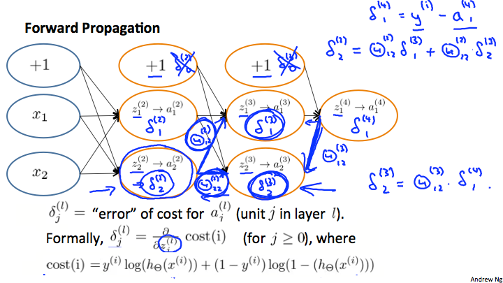
In the image above, to calculate $\delta_2^{(2)}$, we multiply the weights $\Theta_{12}^{(2)}$ and $\Theta_{22}^{(2)}$ by their respective $\delta$ values found to the right of each edge. So we get $\delta_2^{(2)} = \Theta_{12}^{(2)}*\delta_1^{(3)}+\Theta_{22}^{(2)}*\delta_2^{(3)}$. To calculate every single possible $\delta_j^{(l)}$, we could start from the right of our diagram. We can think of our edges as our $\Theta_{ij}$. Going from right to left, to calculate the value of $\delta_j^{(l)}$, you can just take the over all sum of each weight times the $\delta$ it is coming from. Hence, another example would be $\delta_2^{(3)}$ =$\Theta_{12}^{(3)}*\delta_1^{(4)}$.

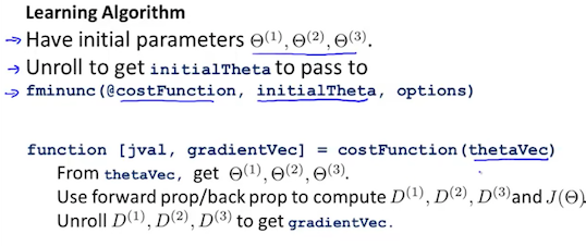
2) Backpropagation in Practice

Implementation Note: Unrolling Parameters

With neural networks, we are working with sets of matrices:

$$
\begin{align*} \Theta^{(1)}, \Theta^{(2)}, \Theta^{(3)}, \dots \newline D^{(1)}, D^{(2)}, D^{(3)}, \dots \end{align*}
$$
In order to use optimizing functions such as "fminunc()", we will want to "unroll" all the elements and put them into one long vector:

thetaVector = [ Theta1(:); Theta2(:); Theta3(:); ]
deltaVector = [ D1(:); D2(:); D3(:) ]

If the dimensions of Theta1 is 10x11, Theta2 is 10x11 and Theta3 is 1x11, then we can get back our original matrices from the "unrolled" versions as follows:

Theta1 = reshape(thetaVector(1:110),10,11)
Theta2 = reshape(thetaVector(111:220),10,11)
Theta3 = reshape(thetaVector(221:231),1,11)

To summarize:

Gradient Checking

Gradient checking will assure that our backpropagation works as intended. We can approximate the derivative of our cost function with:

$$\dfrac{\partial}{\partial\Theta}J(\Theta) \approx \dfrac{J(\Theta + \epsilon) - J(\Theta - \epsilon)}{2\epsilon}$$

With multiple theta matrices, we can approximate the derivative with respect to $Θ_j$ as follows:

$$\dfrac{\partial}{\partial\Theta_j}J(\Theta) \approx \dfrac{J(\Theta_1, \dots, \Theta_j + \epsilon, \dots, \Theta_n) - J(\Theta_1, \dots, \Theta_j - \epsilon, \dots, \Theta_n)}{2\epsilon}$$

A small value for ${\epsilon}$ (epsilon) such as ${\epsilon = 10^{-4}}$, guarantees that the math works out properly. If the value for $\epsilon$ is too small, we can end up with numerical problems.

Hence, we are only adding or subtracting epsilon to the $\Theta_j$ matrix. In octave we can do it as follows:

epsilon = 1e-4;
for i = 1:n,
  thetaPlus = theta;
  thetaPlus(i) += epsilon;
  thetaMinus = theta;
  thetaMinus(i) -= epsilon;
  gradApprox(i) = (J(thetaPlus) - J(thetaMinus))/(2*epsilon)
end;

We previously saw how to calculate the deltaVector. So once we compute our gradApprox vector, we can check that gradApprox ≈ deltaVector.

Once you have verified once that your backpropagation algorithm is correct, you don't need to compute gradApprox again. The code to compute gradApprox can be very slow.

Random Initialization

Why do we need Random Initialization ?
神经网络权重初始化问题 - marsggbo - 博客园 (cnblogs.com)

Initializing all theta weights to zero does not work with neural networks. When we backpropagate, all nodes will update to the same value repeatedly. Instead we can randomly initialize our weights for our $\Theta$ matrices using the following method:

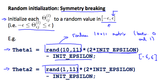
Hence, we initialize each $\Theta^{(l)}_{ij}$ to a random value between $[-\epsilon,\epsilon]$. Using the above formula guarantees that we get the desired bound. The same procedure applies to all the $\Theta$'s. Below is some working code you could use to experiment.

If the dimensions of Theta1 is 10x11, Theta2 is 10x11 and Theta3 is 1x11.

Theta1 = rand(10,11) * (2 * INIT_EPSILON) - INIT_EPSILON;
Theta2 = rand(10,11) * (2 * INIT_EPSILON) - INIT_EPSILON;
Theta3 = rand(1,11) * (2 * INIT_EPSILON) - INIT_EPSILON;

$rand(x,y)$ is just a function in octave that will initialize a matrix of random real numbers between 0 and 1.

(Note: the epsilon used above is unrelated to the epsilon from Gradient Checking)

Putting it Together

First, pick a network architecture; choose the layout of your neural network, including how many hidden units in each layer and how many layers in total you want to have.

• Number of input units = dimension of features $x^{(i)}$

• Number of output units = number of classes

• Number of hidden units per layer = usually more the better (must balance with cost of computation as it increases with more hidden units)

• Defaults: 1 hidden layer. If you have more than 1 hidden layer, then it is recommended that you have the same number of units in every hidden layer.

Training a Neural Network

1. Randomly initialize the weights

2. Implement forward propagation to get $h_\Theta(x^{(i)})$ for any $x^{(i)}$

3. Implement the cost function

4. Implement backpropagation to compute partial derivatives

5. Use gradient checking to confirm that your backpropagation works. Then disable gradient checking.

6. Use gradient descent or a built-in optimization function to minimize the cost function with the weights in theta.

When we perform forward and back propagation, we loop on every training example:

for i = 1:m,
   Perform forward propagation and backpropagation using example (x(i),y(i))
   (Get activations a(l) and delta terms d(l) for l = 2,...,L

The following image gives us an intuition of what is happening as we are implementing our neural network:

Ideally, you want $h_\Theta(x^{(i)})$ $\approx y^{(i)}$ . This will minimize our cost function. However, keep in mind that J (\Theta) J (Θ) is not convex and thus we can end up in a local minimum instead.

11. Advice for Applying Machine Learning

Evaluating a Learning Algorithm

Evaluating a Hypothesis

Once we have done some trouble shooting for errors in our predictions by:

• Getting more training examples

• Trying smaller sets of features

• Trying additional features

• Trying polynomial features

• Increasing or decreasing $\lambda$

We can move on to evaluate our new hypothesis.

A hypothesis may have a low error for the training examples but still be inaccurate (because of overfitting). Thus, to evaluate a hypothesis, given a dataset of training examples, we can split up the data into two sets: a training set and a test set. Typically, the training set consists of 70 % of your data and the test set is the remaining 30 %.

The new procedure using these two sets is then:

1. Learn $\Theta$ and minimize $J_{train}(\Theta)$ using the training set

2. Compute the test set error $J_{test}(\Theta)$

The test set error

1. For linear regression: $J_{test}(\Theta) = \dfrac{1}{2m_{test}} \sum_{i=1}^{m_{test}}(h_\Theta(x^{(i)}{test}) - y^{(i)}{test})^2$

2. For classification ~ Misclassification error (aka 0/1 misclassification error):

$$
err(h_\Theta(x),y) = \begin{matrix} 1 & \mbox{if } h_\Theta(x) \geq 0.5\ and\ y = 0\ or\ h_\Theta(x) < 0.5\ and\ y = 1\newline 0 & \mbox otherwise \end{matrix}
$$

This gives us a binary 0 or 1 error result based on a misclassification. The average test error for the test set is:

$\text{Test Error} = \dfrac{1}{m_{test}} \sum^{m_{test}}{i=1} err(h_\Theta(x^{(i)}{test}), y^{(i)}_{test})$

This gives us the proportion of the test data that was misclassified.

Model Selection and Train/Validation/Test Sets

Just because a learning algorithm fits a training set well, that does not mean it is a good hypothesis. It could over fit and as a result your predictions on the test set would be poor. The error of your hypothesis as measured on the data set with which you trained the parameters will be lower than the error on any other data set.

Given many models with different polynomial degrees, we can use a systematic approach to identify the 'best' function. In order to choose the model of your hypothesis, you can test each degree of polynomial and look at the error result.

One way to break down our dataset into the three sets is:

• Training set: 60%

• Cross validation set: 20%

• Test set: 20%

We can now calculate three separate error values for the three different sets using the following method:

1. Optimize the parameters in Θ using the training set for each polynomial degree.

2. Find the polynomial degree d with the least error using the cross validation set.

3. Estimate the generalization error using the test set with $J_{test}(\Theta^{(d)})$, (d = theta from polynomial with lower error);

This way, the degree of the polynomial d has not been trained using the test set.

Bias vs. Variance

Diagnosing Bias vs. Variance

Why do we need it?
机器学习中的 Bias（偏差）、Error（误差）、Variance（方差）有什么区别和联系？ - 知乎 (zhihu.com)

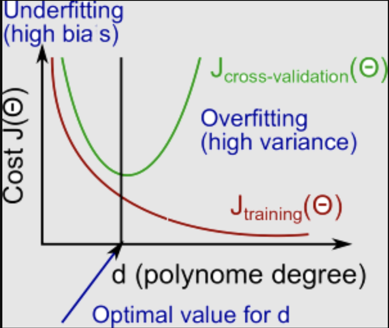
In this section we examine the relationship between the degree of the polynomial d and the underfitting or overfitting of our hypothesis.

• We need to distinguish whether bias or variance is the problem contributing to bad predictions.

• High bias is underfitting and high variance is overfitting. Ideally, we need to find a golden mean between these two.

The training error will tend to decrease as we increase the degree d of the polynomial.

At the same time, the cross validation error will tend to decrease as we increase d up to a point, and then it will increase as d is increased, forming a convex curve.

High bias (underfitting): both $J_{train}(\Theta)$ and $J_{CV}(\Theta)$ will be high. Also, $J_{CV}(\Theta) \approx J_{train}(\Theta)$.

High variance (overfitting): $J_{train}(\Theta)$ will be low and $J_{CV}(\Theta)$ will be much greater than $J_{train}(\Theta)$.

The is summarized in the figure below:

Regularization and Bias/Variance

Note: [The regularization term below and through out the video should be $\frac \lambda {2m} \sum _{j=1}^n \theta_j ^2$ and NOT $\frac \lambda {2m} \sum _{j=1}^m \theta_j ^2$]

In the figure above, we see that as $\lambda$ increases, our fit becomes more rigid. On the other hand, as $\lambda$ approaches 0, we tend to over overfit the data. So how do we choose our parameter $\lambda$ to get it 'just right' ? In order to choose the model and the regularization term $\lambda$, we need to:

1. Create a list of lambdas (i.e. $λ∈{0,0.01,0.02,0.04,0.08,0.16,0.32,0.64,1.28,2.56,5.12,10.24}$);

2. Create a set of models with different degrees or any other variants.

3. Iterate through the $\lambda$ s and for each $\lambda$ go through all the models to learn some $\Theta$ .

4. Compute the cross validation error using the learned $\Theta$ (computed with $\lambda$) on the $J_{CV}(\Theta)$ without regularization or $\lambda = 0$ .

5. Select the best combo that produces the lowest error on the cross validation set.

6. Using the best combo $\Theta$ and $\lambda$, apply it on $J_{test}(\Theta)$ to see if it has a good generalization of the problem.

Learning Curves

Training an algorithm on a very few number of data points (such as 1, 2 or 3) will easily have 0 errors because we can always find a quadratic curve that touches exactly those number of points. Hence:

• As the training set gets larger, the error for a quadratic function increases.

• The error value will plateau out after a certain m, or training set size.

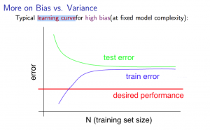
Experiencing high bias:

Low training set size: causes $J_{train}(\Theta)$ to be low and $J_{CV}(\Theta)$ to be high.

Large training set size: causes both $J_{train}(\Theta)$ and $J_{CV}(\Theta)$ to be high with $J_{train}(\Theta) ≈J_{CV}(\Theta)$.

If a learning algorithm is suffering from high bias, getting more training data will not (by itself) help much.

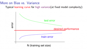
Experiencing high variance:

Low training set size: $J_{train}(\Theta)$ will be low and $J_{CV}(\Theta)$ will be high.

Large training set size: $J_{train}(\Theta)$ increases with training set size and $J_{CV}(\Theta)$ continues to decrease without leveling off. Also, $J_{train}(\Theta) < J_{CV}(\Theta)$ but the difference between them remains significant.

If a learning algorithm is suffering from high variance, getting more training data is likely to help.

Deciding What to Do Next Revisited

Our decision process can be broken down as follows:

• Getting more training examples: Fixes high variance

• Trying smaller sets of features: Fixes high variance

• Adding features: Fixes high bias

• Adding polynomial features: Fixes high bias

• Decreasing λ: Fixes high bias

• Increasing λ: Fixes high variance.

Diagnosing Neural Networks

• A neural network with fewer parameters is prone to underfitting. It is also computationally cheaper.

• A large neural network with more parameters is prone to overfitting. It is also computationally expensive. In this case you can use regularization (increase λ) to address the overfitting.

Using a single hidden layer is a good starting default. You can train your neural network on a number of hidden layers using your cross validation set. You can then select the one that performs best.

Model Complexity Effects:

• Lower-order polynomials (low model complexity) have high bias and low variance. In this case, the model fits poorly consistently.

• Higher-order polynomials (high model complexity) fit the training data extremely well and the test data extremely poorly. These have low bias on the training data, but very high variance.

• In reality, we would want to choose a model somewhere in between, that can generalize well but also fits the data reasonably well.

12. Machine Learning System Design

Building a Spam Classifier

Prioritizing What to Work On

System Design Example:

Given a data set of emails, we could construct a vector for each email. Each entry in this vector represents a word. The vector normally contains 10, 000 to 50, 000 entries gathered by finding the most frequently used words in our data set. If a word is to be found in the email, we would assign its respective entry a 1, else if it is not found, that entry would be a 0. Once we have all our x vectors ready, we train our algorithm and finally, we could use it to classify if an email is a spam or not.

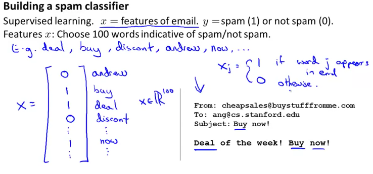
So how could you spend your time to improve the accuracy of this classifier?

• Collect lots of data (for example "honeypot" project but doesn't always work)

• Develop sophisticated features (for example: using email header data in spam emails)

• Develop algorithms to process your input in different ways (recognizing misspellings in spam).

It is difficult to tell which of the options will be most helpful.

Error Analysis

The recommended approach to solving machine learning problems is to:

• Start with a simple algorithm, implement it quickly, and test it early on your cross validation data.

• Plot learning curves to decide if more data, more features, etc. are likely to help.

• Manually examine the errors on examples in the cross validation set and try to spot a trend where most of the errors were made.

For example, assume that we have 500 emails and our algorithm misclassifies a 100 of them. We could manually analyze the 100 emails and categorize them based on what type of emails they are. We could then try to come up with new cues and features that would help us classify these 100 emails correctly. Hence, if most of our misclassified emails are those which try to steal passwords, then we could find some features that are particular to those emails and add them to our model. We could also see how classifying each word according to its root changes our error rate:

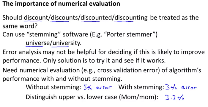
It is very important to get error results as a single, numerical value. Otherwise it is difficult to assess your algorithm's performance. For example if we use stemming, which is the process of treating the same word with different forms (fail/failing/failed) as one word (fail), and get a 3% error rate instead of 5%, then we should definitely add it to our model. However, if we try to distinguish between upper case and lower case letters and end up getting a 3.2% error rate instead of 3%, then we should avoid using this new feature. Hence, we should try new things, get a numerical value for our error rate, and based on our result decide whether we want to keep the new feature or not.

SVM

支持向量机（SVM）——原理篇 - 知乎 (zhihu.com)
svm原理从头到尾详细推导 (qq.com)

[TOC] 十二、支持向量机(Support Vector Machines)

12.1 优化目标

参考视频: 12 - 1 - Optimization Objective (15 min).mkv

到目前为止, 你已经见过一系列不同的学习算法。在监督学习中，许多学习算法的性能都非常类似，因此，重要的不是你该选择使用学习算法A还是学习算法B，而更重要的是，应用这些算法时，所创建的大量数据在应用这些算法时，表现情况通常依赖于你的水平。比如：你为学习算法所设计的特征量的选择，以及如何选择正则化参数，诸如此类的事。还有一个更加强大的算法广泛的应用于工业界和学术界，它被称为支持向量机 (Support Vector Machine)。与逻辑回归和神经网络相比，支持向量机，或者简称SVM，在学习复杂的非线性方程时提供了一种更为清晰，更加强大的方式。因此，在接下来的视频中，我会探讨这一算法。在稍后的课程中，我也会对监督学习算法进行简要的总结。当然，仅仅是作简要描述。但对于支持向量机，鉴于该算法的强大和受欢迎度，在本课中，我会花许多时间来讲解它。它也是我们所介绍的最后一个监督学习算法。

正如我们之前开发的学习算法，我们从优化目标开始。那么，我们开始学习这个算法。为了描述支持向量机，事实上，我将会从逻辑回归开始展示我们如何一点一点修改来得到本质上的支持向量机。

那么，在逻辑回归中我们已经熟悉了这里的假设函数形式，和右边的S型激励函数。然而，为了解释一些数学知识.我将用$z$ 表示$\theta^Tx$。

现在考虑下我们想要逻辑回归做什么：如果有一个 $y=1$的样本，我的意思是不管是在训练集中或是在测试集中，又或者在交叉验证集中，总之是 $y=1$，现在我们希望${{h}{\theta }}\left( x \right)$ 趋近1。因为我们想要正确地将此样本分类，这就意味着当 ${{h}{\theta }}\left( x \right)$趋近于1时，$\theta^Tx$ 应当远大于0，这里的$>>$意思是远远大于0。这是因为由于 $z$ 表示 $\theta^Tx$，当 $z$远大于0时，即到了该图的右边，你不难发现此时逻辑回归的输出将趋近于1。相反地，如果我们有另一个样本，即$y=0$。我们希望假设函数的输出值将趋近于0，这对应于$\theta^Tx$，或者就是 $z$ 会远小于0，因为对应的假设函数的输出值趋近0。

如果你进一步观察逻辑回归的代价函数，你会发现每个样本 $(x,y)$都会为总代价函数，增加这里的一项，因此，对于总代价函数通常会有对所有的训练样本求和，并且这里还有一个$1/m$项，但是，在逻辑回归中，这里的这一项就是表示一个训练样本所对应的表达式。现在，如果我将完整定义的假设函数代入这里。那么，我们就会得到每一个训练样本都影响这一项。

现在，先忽略 $1/m$ 这一项，但是这一项是影响整个总代价函数中的这一项的。

现在，一起来考虑两种情况：

一种是$y$等于1的情况；另一种是 $y$ 等于0的情况。

在第一种情况中，假设 $y=1$ ，此时在目标函数中只需有第一项起作用，因为$y=1$时，$(1-y)$项将等于0。因此，当在 $y=1$ 的样本中时，即在 $(x, y) $中 ，我们得到 $y=1$ $-\log(1-\frac{1}{1+e^{-z}})​$这样一项，这里同上一张幻灯片一致。

我用 $z$ 表示$\theta^Tx$，即： $z= \theta^Tx$。当然，在代价函数中，$y$ 前面有负号。我们只是这样表示，如果 $y=1$ 代价函数中，这一项也等于1。这样做是为了简化此处的表达式。如果画出关于$z$ 的函数，你会看到左下角的这条曲线，我们同样可以看到，当$z$ 增大时，也就是相当于$\theta^Tx$增大时，$z$ 对应的值会变的非常小。对整个代价函数而言，影响也非常小。这也就解释了，为什么逻辑回归在观察到正样本$y=1$时，试图将$\theta^Tx$设置得非常大。因为，在代价函数中的这一项会变的非常小。

现在开始建立支持向量机，我们从这里开始：

我们会从这个代价函数开始，也就是$-\log(1-\frac{1}{1+e^{-z}})$一点一点修改，让我取这里的$z=1$ 点，我先画出将要用的代价函数。

新的代价函数将会水平的从这里到右边(图外)，然后我再画一条同逻辑回归非常相似的直线，但是，在这里是一条直线，也就是我用紫红色画的曲线，就是这条紫红色的曲线。那么，到了这里已经非常接近逻辑回归中使用的代价函数了。只是这里是由两条线段组成，即位于右边的水平部分和位于左边的直线部分，先别过多的考虑左边直线部分的斜率，这并不是很重要。但是，这里我们将使用的新的代价函数，是在$y=1$的前提下的。你也许能想到，这应该能做同逻辑回归中类似的事情，但事实上，在之后的优化问题中，这会变得更坚定，并且为支持向量机，带来计算上的优势。例如，更容易计算股票交易的问题等等。

目前，我们只是讨论了$y=1$的情况，另外一种情况是当$y=0$时，此时如果你仔细观察代价函数只留下了第二项，因为第一项被消除了。如果当$y=0$时，那么这一项也就是0了。所以上述表达式只留下了第二项。因此，这个样本的代价或是代价函数的贡献。将会由这一项表示。并且，如果你将这一项作为$z$的函数，那么，这里就会得到横轴$z$。现在，你完成了支持向量机中的部分内容，同样地，我们要替代这一条蓝色的线，用相似的方法。

如果我们用一个新的代价函数来代替，即这条从0点开始的水平直线，然后是一条斜线，像上图。那么，现在让我给这两个方程命名，左边的函数，我称之为${\cos}t_1{(z)}$，同时，右边函数我称它为${\cos}t_0{(z)}$。这里的下标是指在代价函数中，对应的 $y=1$ 和 $y=0$ 的情况，拥有了这些定义后，现在，我们就开始构建支持向量机。

这是我们在逻辑回归中使用代价函数$J(\theta)$。也许这个方程看起来不是非常熟悉。这是因为之前有个负号在方程外面，但是，这里我所做的是，将负号移到了表达式的里面，这样做使得方程看起来有些不同。对于支持向量机而言，实质上我们要将这替换为${\cos}t_1{(z)}$，也就是${\cos}t_1{(\theta^Tx)}$，同样地，我也将这一项替换为${\cos}t_0{(z)}$，也就是代价${\cos}t_0{(\theta^Tx)}$。这里的代价函数${\cos}t_1$，就是之前所提到的那条线。此外，代价函数${\cos}t_0$，也是上面所介绍过的那条线。因此，对于支持向量机，我们得到了这里的最小化问题，即:

然后，再加上正则化参数。现在，按照支持向量机的惯例，事实上，我们的书写会稍微有些不同，代价函数的参数表示也会稍微有些不同。

首先，我们要除去$1/m$这一项，当然，这仅仅是由于人们使用支持向量机时，对比于逻辑回归而言，不同的习惯所致，但这里我所说的意思是：你知道，我将要做的是仅仅除去$1/m$这一项，但是，这也会得出同样的 ${{\theta }}$ 最优值，好的，因为$1/m$ 仅是个常量，因此，你知道在这个最小化问题中，无论前面是否有$1/m$ 这一项，最终我所得到的最优值${{\theta }}$都是一样的。这里我的意思是，先给你举一个样本，假定有一最小化问题：即要求当$(u-5)^2+1$取得最小值时的$u$值，这时最小值为：当$u=5$时取得最小值。

现在，如果我们想要将这个目标函数乘上常数10，这里我的最小化问题就变成了：求使得$10×(u-5)^2+10$最小的值$u$，然而，使得这里最小的$u$值仍为5。因此将一些常数乘以你的最小化项，这并不会改变最小化该方程时得到$u$值。因此，这里我所做的是删去常量$m$。也相同的，我将目标函数乘上一个常量$m$，并不会改变取得最小值时的${{\theta }}$值。

第二点概念上的变化，我们只是指在使用支持向量机时，一些如下的标准惯例，而不是逻辑回归。因此，对于逻辑回归，在目标函数中，我们有两项：第一个是训练样本的代价，第二个是我们的正则化项，我们不得不去用这一项来平衡。这就相当于我们想要最小化$A$加上正则化参数$\lambda$，然后乘以其他项$B$对吧？这里的$A$表示这里的第一项，同时我用B表示第二项，但不包括$\lambda$，我们不是优化这里的$A+\lambda\times B$。我们所做的是通过设置不同正则参数$\lambda$达到优化目的。这样，我们就能够权衡对应的项，是使得训练样本拟合的更好。即最小化$A$。还是保证正则参数足够小，也即是对于B项而言，但对于支持向量机，按照惯例，我们将使用一个不同的参数替换这里使用的$\lambda$来权衡这两项。你知道，就是第一项和第二项我们依照惯例使用一个不同的参数称为$C$，同时改为优化目标，$C×A+B$。 因此，在逻辑回归中，如果给定$\lambda$，一个非常大的值，意味着给予$B$更大的权重。而这里，就对应于将$C$ 设定为非常小的值，那么，相应的将会给$B$比给$A$更大的权重。因此，这只是一种不同的方式来控制这种权衡或者一种不同的方法，即用参数来决定是更关心第一项的优化，还是更关心第二项的优化。当然你也可以把这里的参数$C$ 考虑成$1/\lambda$，同 $1/\lambda$所扮演的角色相同，并且这两个方程或这两个表达式并不相同，因为$C=1/\lambda$，但是也并不全是这样，如果当$C=1/\lambda$时，这两个优化目标应当得到相同的值，相同的最优值 ${{\theta }}$。因此，就用它们来代替。那么，我现在删掉这里的$\lambda$，并且用常数$C$来代替。因此，这就得到了在支持向量机中我们的整个优化目标函数。然后最小化这个目标函数，得到SVM 学习到的参数$C$。

最后有别于逻辑回归输出的概率。在这里，我们的代价函数，当最小化代价函数，获得参数${{\theta }}$时，支持向量机所做的是它来直接预测$y$的值等于1，还是等于0。因此，这个假设函数会预测1。当$\theta^Tx$大于或者等于0时，或者等于0时，所以学习参数${{\theta }}$就是支持向量机假设函数的形式。那么，这就是支持向量机数学上的定义。

在接下来的视频中，让我们再回去从直观的角度看看优化目标，实际上是在做什么，以及SVM的假设函数将会学习什么，同时也会谈谈如何做些许修改，学习更加复杂、非线性的函数。

12.2 大边界的直观理解

参考视频: 12 - 2 - Large Margin Intuition (11 min).mkv

人们有时将支持向量机看作是大间距分类器。在这一部分，我将介绍其中的含义，这有助于我们直观理解SVM模型的假设是什么样的。

这是我的支持向量机模型的代价函数，在左边这里我画出了关于$z$的代价函数${\cos}t_1{(z)}$，此函数用于正样本，而在右边这里我画出了关于$z$的代价函数${\cos}t_0{(z)}$，横轴表示$z$，现在让我们考虑一下，最小化这些代价函数的必要条件是什么。如果你有一个正样本，$y=1$，则只有在$z>=1$时，代价函数${\cos}t_1{(z)}$才等于0。

换句话说，如果你有一个正样本，我们会希望$\theta^Tx>=1$，反之，如果$y=0$，我们观察一下，函数${\cos}t_0{(z)}$，它只有在$z<=-1$的区间里函数值为0。这是支持向量机的一个有趣性质。事实上，如果你有一个正样本$y=1$，则其实我们仅仅要求$\theta^Tx$大于等于0，就能将该样本恰当分出，这是因为如果$\theta^Tx$>0大的话，我们的模型代价函数值为0，类似地，如果你有一个负样本，则仅需要$\theta^Tx$<=0就会将负例正确分离，但是，支持向量机的要求更高，不仅仅要能正确分开输入的样本，即不仅仅要求$\theta^Tx$>0，我们需要的是比0值大很多，比如大于等于1，我也想这个比0小很多，比如我希望它小于等于-1，这就相当于在支持向量机中嵌入了一个额外的安全因子，或者说安全的间距因子。

当然，逻辑回归做了类似的事情。但是让我们看一下，在支持向量机中，这个因子会导致什么结果。具体而言，我接下来会考虑一个特例。我们将这个常数$C$设置成一个非常大的值。比如我们假设$C$的值为100000或者其它非常大的数，然后来观察支持向量机会给出什么结果？

如果 $C$非常大，则最小化代价函数的时候，我们将会很希望找到一个使第一项为0的最优解。因此，让我们尝试在代价项的第一项为0的情形下理解该优化问题。比如我们可以把$C$设置成了非常大的常数，这将给我们一些关于支持向量机模型的直观感受。

$\min_\limits{\theta}C\sum_\limits{i=1}^{m}\left[y^{(i)}{\cos}t_{1}\left(\theta^{T}x^{(i)}\right)+\left(1-y^{(i)}\right){\cos}t\left(\theta^{T}x^{(i)}\right)\right]+\frac{1}{2}\sum_\limits{i=1}^{n}\theta^{2}_{j}$

我们已经看到输入一个训练样本标签为$y=1​$，你想令第一项为0，你需要做的是找到一个${{\theta }}​$，使得$\theta^Tx>=1​$，类似地，对于一个训练样本，标签为$y=0​$，为了使${\cos}t_0{(z)}​$ 函数的值为0，我们需要$\theta^Tx<=-1​$。因此，现在考虑我们的优化问题。选择参数，使得第一项等于0，就会导致下面的优化问题，因为我们将选择参数使第一项为0，因此这个函数的第一项为0，因此是$C​$乘以0加上二分之一乘以第二项。这里第一项是$C​$乘以0，因此可以将其删去，因为我知道它是0。

这将遵从以下的约束：$\theta^Tx^{(i)}>=1$，如果 $y^{(i)}$是等于1 的，$\theta^Tx^{(i)}<=-1$，如果样本$i$是一个负样本，这样当你求解这个优化问题的时候，当你最小化这个关于变量${{\theta }}$的函数的时候，你会得到一个非常有趣的决策边界。

具体而言，如果你考察这样一个数据集，其中有正样本，也有负样本，可以看到这个数据集是线性可分的。我的意思是，存在一条直线把正负样本分开。当然有多条不同的直线，可以把正样本和负样本完全分开。

比如，这就是一个决策边界可以把正样本和负样本分开。但是多多少少这个看起来并不是非常自然是么?

或者我们可以画一条更差的决策界，这是另一条决策边界，可以将正样本和负样本分开，但仅仅是勉强分开，这些决策边界看起来都不是特别好的选择，支持向量机将会选择这个黑色的决策边界，相较于之前我用粉色或者绿色画的决策界。这条黑色的看起来好得多，黑线看起来是更稳健的决策界。在分离正样本和负样本上它显得的更好。数学上来讲，这是什么意思呢？这条黑线有更大的距离，这个距离叫做间距(margin)。

当画出这两条额外的蓝线，我们看到黑色的决策界和训练样本之间有更大的最短距离。然而粉线和蓝线离训练样本就非常近，在分离样本的时候就会比黑线表现差。因此，这个距离叫做支持向量机的间距，而这是支持向量机具有鲁棒性的原因，因为它努力用一个最大间距来分离样本。因此支持向量机有时被称为大间距分类器，而这其实是求解上一页幻灯片上优化问题的结果。

我知道你也许想知道求解上一页幻灯片中的优化问题为什么会产生这个结果？它是如何产生这个大间距分类器的呢？我知道我还没有解释这一点。

我将会从直观上略述为什么这个优化问题会产生大间距分类器。总之这个图示有助于你理解支持向量机模型的做法，即努力将正样本和负样本用最大的间距分开。

在本节课中关于大间距分类器，我想讲最后一点：我们将这个大间距分类器中的正则化因子常数$C$设置的非常大，我记得我将其设置为了100000，因此对这样的一个数据集，也许我们将选择这样的决策界，从而最大间距地分离开正样本和负样本。那么在让代价函数最小化的过程中，我们希望找出在$y=1$和$y=0$两种情况下都使得代价函数中左边的这一项尽量为零的参数。如果我们找到了这样的参数，则我们的最小化问题便转变成：

事实上，支持向量机现在要比这个大间距分类器所体现得更成熟，尤其是当你使用大间距分类器的时候，你的学习算法会受异常点(outlier) 的影响。比如我们加入一个额外的正样本。

在这里，如果你加了这个样本，为了将样本用最大间距分开，也许我最终会得到一条类似这样的决策界，对么？就是这条粉色的线，仅仅基于一个异常值，仅仅基于一个样本，就将我的决策界从这条黑线变到这条粉线，这实在是不明智的。而如果正则化参数$C$，设置的非常大，这事实上正是支持向量机将会做的。它将决策界，从黑线变到了粉线，但是如果$C$ 设置的小一点，如果你将C设置的不要太大，则你最终会得到这条黑线，当然数据如果不是线性可分的，如果你在这里有一些正样本或者你在这里有一些负样本，则支持向量机也会将它们恰当分开。因此，大间距分类器的描述，仅仅是从直观上给出了正则化参数$C$非常大的情形，同时，要提醒你$C$的作用类似于$1/\lambda$，$\lambda$是我们之前使用过的正则化参数。这只是$C$非常大的情形，或者等价地 $\lambda$ 非常小的情形。你最终会得到类似粉线这样的决策界，但是实际上应用支持向量机的时候，当$C$不是非常非常大的时候，它可以忽略掉一些异常点的影响，得到更好的决策界。甚至当你的数据不是线性可分的时候，支持向量机也可以给出好的结果。

回顾 $C=1/\lambda$，因此：

$C$ 较大时，相当于 $\lambda$ 较小，可能会导致过拟合，高方差。

$C$ 较小时，相当于$\lambda$较大，可能会导致低拟合，高偏差。

我们稍后会介绍支持向量机的偏差和方差，希望在那时候关于如何处理参数的这种平衡会变得更加清晰。我希望，这节课给出了一些关于为什么支持向量机被看做大间距分类器的直观理解。它用最大间距将样本区分开，尽管从技术上讲，这只有当参数$C$是非常大的时候是真的，但是它对于理解支持向量机是有益的。

本节课中我们略去了一步，那就是我们在幻灯片中给出的优化问题。为什么会是这样的？它是如何得出大间距分类器的？我在本节中没有讲解，在下一节课中，我将略述这些问题背后的数学原理，来解释这个优化问题是如何得到一个大间距分类器的。

12.3 大边界分类背后的数学（选修）

参考视频: 12 - 3 - Mathematics Behind Large Margin Classification (Optional) (20 min).mkv

在本节课中，我将介绍一些大间隔分类背后的数学原理。本节为选修部分，你完全可以跳过它，但是听听这节课可能让你对支持向量机中的优化问题，以及如何得到大间距分类器，产生更好的直观理解。

首先，让我来给大家复习一下关于向量内积的知识。假设我有两个向量，$u$和$v$，我将它们写在这里。两个都是二维向量，我们看一下，$u^T v$的结果。$u^T v$也叫做向量$u$和$v$之间的内积。由于是二维向量，我可以将它们画在这个图上。我们说，这就是向量$u$即在横轴上，取值为某个${{u}{1}}$，而在纵轴上，高度是某个${{u}{2}}$作为$u$的第二个分量。现在，很容易计算的一个量就是向量$u$的范数。$\left| u \right|$表示$u$的范数，即$u$的长度，即向量$u$的欧几里得长度。根据毕达哥拉斯定理，$\left| u \right|=\sqrt{u_{1}^{2}+u_{2}^{2}}$，这是向量$u$的长度，它是一个实数。现在你知道了这个的长度是多少了。我刚刚画的这个向量的长度就知道了。

现在让我们回头来看向量$v$ ，因为我们想计算内积。$v$是另一个向量，它的两个分量${{v}{1}}$和${{v}{2}}$是已知的。向量$v$可以画在这里，现在让我们来看看如何计算$u$和$v$之间的内积。这就是具体做法，我们将向量$v$投影到向量$u$上，我们做一个直角投影，或者说一个90度投影将其投影到$u$上，接下来我度量这条红线的长度。我称这条红线的长度为$p$，因此$p$就是长度，或者说是向量$v$投影到向量$u$上的量，我将它写下来，$p$是$v$投影到向量$u$上的长度，因此可以将${{u}^{T}}v=p\centerdot \left| u \right|$，或者说$u$的长度。这是计算内积的一种方法。如果你从几何上画出$p$的值，同时画出$u$的范数，你也会同样地计算出内积，答案是一样的。另一个计算公式是：$u^T v$就是$\left[ {{u}{1}}\text{ }{{u}{2}} \right]$ 这个一行两列的矩阵乘以$v$。因此可以得到${{u}{1}}\times {{v}{1}}+{{u}{2}}\times {{v}{2}}$。根据线性代数的知识，这两个公式会给出同样的结果。顺便说一句，$u^Tv=v^Tu$。因此如果你将$u$和$v$交换位置，将$u$投影到$v$上，而不是将$v$投影到$u$上，然后做同样地计算，只是把$u$和$v$的位置交换一下，你事实上可以得到同样的结果。申明一点，在这个等式中$u$的范数是一个实数，$p$也是一个实数，因此$u^T v$就是两个实数正常相乘。

最后一点，需要注意的就是$p$值，$p$事实上是有符号的，即它可能是正值，也可能是负值。我的意思是说，如果$u$是一个类似这样的向量，$v$是一个类似这样的向量，$u$和$v$之间的夹角大于90度，则如果将$v$投影到$u$上，会得到这样的一个投影，这是$p$的长度，在这个情形下我们仍然有${{u}^{T}}v$是等于$p$乘以$u$的范数。唯一一点不同的是$p$在这里是负的。在内积计算中，如果$u$和$v$之间的夹角小于90度，那么那条红线的长度$p$是正值。然而如果这个夹角大于90度，则$p$将会是负的。就是这个小线段的长度是负的。如果它们之间的夹角大于90度，两个向量之间的内积也是负的。这就是关于向量内积的知识。我们接下来将会使用这些关于向量内积的性质试图来理解支持向量机中的目标函数。

这就是我们先前给出的支持向量机模型中的目标函数。为了讲解方便，我做一点简化，仅仅是为了让目标函数更容易被分析。

我接下来忽略掉截距，令${{\theta }{0}}=0$，这样更容易画示意图。我将特征数$n$置为2，因此我们仅有两个特征${{x}{1}},{{x}{2}}$，现在我们来看一下目标函数，支持向量机的优化目标函数。当我们仅有两个特征，即$n=2$时，这个式子可以写作：$\frac{1}{2}\left({\theta_1^2+\theta_2^2}\right)=\frac{1}{2}\left(\sqrt{\theta_1^2+\theta_2^2}\right)^2$，我们只有两个参数${{\theta }{1}},{{\theta }_{2}}$。你可能注意到括号里面的这一项是向量${{\theta }}$的范数，或者说是向量${{\theta }}$的长度。我的意思是如果我们将向量${{\theta }}$写出来，那么我刚刚画红线的这一项就是向量${{\theta }}$的长度或范数。这里我们用的是之前学过的向量范数的定义，事实上这就等于向量${{\theta }}$的长度。

当然你可以将其写作${{\theta }{0}}\text{,}{{\theta }{1}},{{\theta }{2}}$，如果${{\theta }{0}}=0$，那就是${{\theta }{1}},{{\theta }{2}}$的长度。在这里我将忽略${{\theta }{0}}$，这样来写$\theta$的范数，它仅仅和${{\theta }{1}},{{\theta }{2}}$有关。但是，数学上不管你是否包含，其实并没有差别，因此在我们接下来的推导中去掉${{\theta }{0}}$不会有影响这意味着我们的目标函数是等于$\frac{1}{2}\left| \theta \right|^2$。因此支持向量机做的全部事情，就是极小化参数向量${{\theta }}$范数的平方，或者说长度的平方。

现在我将要看看这些项：$\theta^{T}x$更深入地理解它们的含义。给定参数向量$\theta $给定一个样本$x$，这等于什么呢?在前一页幻灯片上，我们画出了在不同情形下，$u^Tv$的示意图，我们将会使用这些概念，$\theta $和$x^{(i)}$就类似于$u$和$v$ 。

让我们看一下示意图：我们考察一个单一的训练样本，我有一个正样本在这里，用一个叉来表示这个样本$x^{(i)}​$，意思是在水平轴上取值为$x_1^{(i)}​$，在竖直轴上取值为$x_2^{(i)}​$。这就是我画出的训练样本。尽管我没有将其真的看做向量。它事实上就是一个始于原点，终点位置在这个训练样本点的向量。现在，我们有一个参数向量我会将它也画成向量。我将$θ_1​$画在横轴这里，将$θ_2​$ 画在纵轴这里，那么内积$θ^T x^{(i)}$ 将会是什么呢？

使用我们之前的方法，我们计算的方式就是我将训练样本投影到参数向量${{\theta }}$，然后我来看一看这个线段的长度，我将它画成红色。我将它称为$p^{(i)}$用来表示这是第 $i$个训练样本在参数向量${{\theta }}$上的投影。根据我们之前幻灯片的内容，我们知道的是$θ^Tx^{(i)}$将会等于$p$ 乘以向量 $θ$ 的长度或范数。这就等于$\theta_1\cdot{x_1^{(i)}}+\theta_2\cdot{x_2^{(i)}}$。这两种方式是等价的，都可以用来计算$θ$和$x^{(i)}$之间的内积。

这告诉了我们什么呢？这里表达的意思是：这个$θ^Tx^{(i)}>=1$ 或者$θ^Tx^{(i)}<-1$的,约束是可以被$p^{(i)}\cdot{x}>=1$这个约束所代替的。因为$θ^Tx^{(i)}=p^{(i)}\cdot{\left| \theta \right|}$ ，将其写入我们的优化目标。我们将会得到没有了约束，$θ^Tx^{(i)}$而变成了$p^{(i)}\cdot{\left| \theta \right|}$。

需要提醒一点，我们之前曾讲过这个优化目标函数可以被写成等于$\frac{1}{2}\left| \theta \right|^2$。

现在让我们考虑下面这里的训练样本。现在，继续使用之前的简化，即${{\theta }_{0}}=0$，我们来看一下支持向量机会选择什么样的决策界。这是一种选择，我们假设支持向量机会选择这个决策边界。这不是一个非常好的选择，因为它的间距很小。这个决策界离训练样本的距离很近。我们来看一下为什么支持向量机不会选择它。

对于这样选择的参数${{\theta }}$，可以看到参数向量${{\theta }}$事实上是和决策界是90度正交的，因此这个绿色的决策界对应着一个参数向量${{\theta }}$这个方向,顺便提一句${{\theta }_{0}}=0$的简化仅仅意味着决策界必须通过原点$(0,0)$。现在让我们看一下这对于优化目标函数意味着什么。

比如这个样本，我们假设它是我的第一个样本$x^{(1)}$，如果我考察这个样本到参数${{\theta }}$的投影，投影是这个短的红线段，就等于$p^{(1)}$，它非常短。类似地，这个样本如果它恰好是$x^{(2)}$，我的第二个训练样本，则它到${{\theta }}$的投影在这里。我将它画成粉色，这个短的粉色线段是$p^{(2)}$，即第二个样本到我的参数向量${{\theta }}$的投影。因此，这个投影非常短。$p^{(2)}$事实上是一个负值，$p^{(2)}$是在相反的方向，这个向量和参数向量${{\theta }}$的夹角大于90度，$p^{(2)}$的值小于0。

我们会发现这些$p^{(i)}$将会是非常小的数，因此当我们考察优化目标函数的时候，对于正样本而言，我们需要$p^{(i)}\cdot{\left| \theta \right|}>=1$,但是如果 $p^{(i)}$在这里非常小,那就意味着我们需要${{\theta }}$的范数非常大.因为如果 $p^{(1)}$ 很小,而我们希望$p^{(1)}\cdot{\left| \theta \right|}>=1$,令其实现的唯一的办法就是这两个数较大。如果 $p^{(1)}$ 小，我们就希望${{\theta }}$的范数大。类似地，对于负样本而言我们需要$p^{(2)}\cdot{\left|\theta \right|}<=-1$。我们已经在这个样本中看到$p^{(2)}$会是一个非常小的数，因此唯一的办法就是${{\theta }}$的范数变大。但是我们的目标函数是希望找到一个参数${{\theta }}$，它的范数是小的。因此，这看起来不像是一个好的参数向量${{\theta }}$的选择。

相反的，来看一个不同的决策边界。比如说，支持向量机选择了这个决策界，现在状况会有很大不同。如果这是决策界，这就是相对应的参数${{\theta }}$的方向，因此，在这个决策界之下，垂直线是决策界。使用线性代数的知识，可以说明，这个绿色的决策界有一个垂直于它的向量${{\theta }}$。现在如果你考察你的数据在横轴$x$上的投影，比如这个我之前提到的样本，我的样本$x^{(1)}$，当我将它投影到横轴$x$上，或说投影到${{\theta }}$上，就会得到这样$p^{(1)}$。它的长度是$p^{(1)}$，另一个样本，那个样本是$x^{(2)}$。我做同样的投影，我会发现，$p^{(2)}$的长度是负值。你会注意到现在$p^{(1)}$ 和$p^{(2)}$这些投影长度是长多了。如果我们仍然要满足这些约束，$P^{(i)}\cdot{\left| \theta \right|}$>1，则因为$p^{(1)}$变大了，${{\theta }}$的范数就可以变小了。因此这意味着通过选择右边的决策界，而不是左边的那个，支持向量机可以使参数${{\theta }}$的范数变小很多。因此，如果我们想令${{\theta }}$的范数变小，从而令${{\theta }}$范数的平方变小，就能让支持向量机选择右边的决策界。这就是支持向量机如何能有效地产生大间距分类的原因。

看这条绿线，这个绿色的决策界。我们希望正样本和负样本投影到$\theta$的值大。要做到这一点的唯一方式就是选择这条绿线做决策界。这是大间距决策界来区分开正样本和负样本这个间距的值。这个间距的值就是$p^{(1)},p^{(2)},p^{(3)}$等等的值。通过让间距变大，即通过这些$p^{(1)},p^{(2)},p^{(3)}$等等的值，支持向量机最终可以找到一个较小的${{\theta }}$范数。这正是支持向量机中最小化目标函数的目的。

以上就是为什么支持向量机最终会找到大间距分类器的原因。因为它试图极大化这些$p^{(i)}$的范数，它们是训练样本到决策边界的距离。最后一点，我们的推导自始至终使用了这个简化假设，就是参数$θ_0=0$。

就像我之前提到的。这个的作用是：$θ_0=0$的意思是我们让决策界通过原点。如果你令$θ_0$不是0的话，含义就是你希望决策界不通过原点。我将不会做全部的推导。实际上，支持向量机产生大间距分类器的结论，会被证明同样成立，证明方式是非常类似的，是我们刚刚做的证明的推广。

之前视频中说过，即便$θ_0$不等于0，支持向量机要做的事情都是优化这个目标函数对应着$C$值非常大的情况，但是可以说明的是，即便$θ_0$不等于0，支持向量机仍然会找到正样本和负样本之间的大间距分隔。

总之，我们解释了为什么支持向量机是一个大间距分类器。在下一节我们，将开始讨论如何利用支持向量机的原理，应用它们建立一个复杂的非线性分类器。

12.4 核函数1

参考视频: 12 - 4 - Kernels I (16 min).mkv

回顾我们之前讨论过可以使用高级数的多项式模型来解决无法用直线进行分隔的分类问题：

为了获得上图所示的判定边界，我们的模型可能是 ${{\theta }{0}}+{{\theta }{1}}{{x}{1}}+{{\theta }{2}}{{x}{2}}+{{\theta }{3}}{{x}{1}}{{x}{2}}+{{\theta }{4}}x{1}^{2}+{{\theta }{5}}x{2}^{2}+\cdots=$ 的形式。

我们可以用一系列的新的特征$f$来替换模型中的每一项。例如令： ${{f}{1}}={{x}{1}},{{f}{2}}={{x}{2}},{{f}{3}}={{x}{1}}{{x}{2}},{{f}{4}}=x_{1}^{2},{{f}{5}}=x{2}^{2}$

...得到$h_θ(x)={{\theta }{1}}f_1+{{\theta }{2}}f_2+...+{{\theta }_{n}}f_n$。然而，除了对原有的特征进行组合以外，有没有更好的方法来构造$f_1,f_2,f_3$？我们可以利用核函数来计算出新的特征。

给定一个训练样本$x$，我们利用$x$的各个特征与我们预先选定的地标(landmarks)$l^{(1)},l^{(2)},l^{(3)}$的近似程度来选取新的特征$f_1,f_2,f_3$。

例如：${{f}_{1}}=similarity(x,{{l}^{(1)}})=e(-\frac{{{\left| x-{{l}^{(1)}} \right|}^{2}}}{2{{\sigma }^{2}}})$

其中：${{\left| x-{{l}^{(1)}} \right|}^{2}}=\sum{{j=1}^{n}}{{({{x}{j}}-l_{j}^{(1)})}^{2}}$，为实例$x$中所有特征与地标$l^{(1)}$之间的距离的和。上例中的$similarity(x,{{l}^{(1)}})$就是核函数，具体而言，这里是一个高斯核函数(Gaussian Kernel)。 注：这个函数与正态分布没什么实际上的关系，只是看上去像而已。

这些地标的作用是什么？如果一个训练样本$x$与地标$l$之间的距离近似于0，则新特征 $f$近似于$e^{-0}=1$，如果训练样本$x$与地标$l$之间距离较远，则$f$近似于$e^{-(一个较大的数)}=0$。

假设我们的训练样本含有两个特征[$x_{1}$ $x{_2}$]，给定地标$l^{(1)}$与不同的$\sigma$值，见下图：

图中水平面的坐标为 $x_{1}$，$x_{2}$而垂直坐标轴代表$f$。可以看出，只有当$x$与$l^{(1)}$重合时$f$才具有最大值。随着$x$的改变$f$值改变的速率受到$\sigma^2$的控制。

在下图中，当样本处于洋红色的点位置处，因为其离$l^{(1)}$更近，但是离$l^{(2)}$和$l^{(3)}$较远，因此$f_1$接近1，而$f_2$,$f_3$接近0。因此$h_θ(x)=θ_0+θ_1f_1+θ_2f_2+θ_1f_3>0$，因此预测$y=1$。同理可以求出，对于离$l^{(2)}$较近的绿色点，也预测$y=1$，但是对于蓝绿色的点，因为其离三个地标都较远，预测$y=0$。

这样，图中红色的封闭曲线所表示的范围，便是我们依据一个单一的训练样本和我们选取的地标所得出的判定边界，在预测时，我们采用的特征不是训练样本本身的特征，而是通过核函数计算出的新特征$f_1,f_2,f_3$。

12.5 核函数2

参考视频: 12 - 5 - Kernels II (16 min).mkv

在上一节视频里，我们讨论了核函数这个想法，以及怎样利用它去实现支持向量机的一些新特性。在这一节视频中，我将补充一些缺失的细节，并简单的介绍一下怎么在实际中使用应用这些想法。

如何选择地标？

我们通常是根据训练集的数量选择地标的数量，即如果训练集中有$m$个样本，则我们选取$m$个地标，并且令:$l^{(1)}=x^{(1)},l^{(2)}=x^{(2)},.....,l^{(m)}=x^{(m)}$。这样做的好处在于：现在我们得到的新特征是建立在原有特征与训练集中所有其他特征之间距离的基础之上的，即：

下面我们将核函数运用到支持向量机中，修改我们的支持向量机假设为：

• 给定$x$，计算新特征$f$，当$θ^Tf>=0$ 时，预测 $y=1$，否则反之。

相应地修改代价函数为：$\sum{_{j=1}^{n=m}}\theta _{j}^{2}={{\theta}^{T}}\theta $，

$min C\sum\limits_{i=1}^{m}{[{{y}^{(i)}}cos {{t}{1}}}( {{\theta }^{T}}{{f}^{(i)}})+(1-{{y}^{(i)}})cos {{t}{0}}( {{\theta }^{T}}{{f}^{(i)}})]+\frac{1}{2}\sum\limits_{j=1}^{n=m}{\theta {j}^{2}}$ 在具体实施过程中，我们还需要对最后的正则化项进行些微调整，在计算$\sum{{j=1}^{n=m}}\theta _{j}^{2}={{\theta}^{T}}\theta $时，我们用$θ^TMθ$代替$θ^Tθ$，其中$M$是根据我们选择的核函数而不同的一个矩阵。这样做的原因是为了简化计算。

理论上讲，我们也可以在逻辑回归中使用核函数，但是上面使用 $M$来简化计算的方法不适用与逻辑回归，因此计算将非常耗费时间。

在此，我们不介绍最小化支持向量机的代价函数的方法，你可以使用现有的软件包（如liblinear,libsvm等）。在使用这些软件包最小化我们的代价函数之前，我们通常需要编写核函数，并且如果我们使用高斯核函数，那么在使用之前进行特征缩放是非常必要的。

另外，支持向量机也可以不使用核函数，不使用核函数又称为线性核函数(linear kernel)，当我们不采用非常复杂的函数，或者我们的训练集特征非常多而样本非常少的时候，可以采用这种不带核函数的支持向量机。

下面是支持向量机的两个参数$C$和$\sigma$的影响：

$C=1/\lambda$

$C$ 较大时，相当于$\lambda$较小，可能会导致过拟合，高方差；

$C$ 较小时，相当于$\lambda$较大，可能会导致低拟合，高偏差；

$\sigma$较大时，可能会导致低方差，高偏差；

$\sigma$较小时，可能会导致低偏差，高方差。

如果你看了本周的编程作业，你就能亲自实现这些想法，并亲眼看到这些效果。这就是利用核函数的支持向量机算法，希望这些关于偏差和方差的讨论，能给你一些对于算法结果预期的直观印象。

12.6 使用支持向量机

参考视频: 12 - 6 - Using An SVM (21 min).mkv

目前为止，我们已经讨论了SVM比较抽象的层面，在这个视频中我将要讨论到为了运行或者运用SVM。你实际上所需要的一些东西：支持向量机算法，提出了一个特别优化的问题。但是就如在之前的视频中我简单提到的，我真的不建议你自己写软件来求解参数${{\theta }}$，因此由于今天我们中的很少人，或者其实没有人考虑过自己写代码来转换矩阵，或求一个数的平方根等我们只是知道如何去调用库函数来实现这些功能。同样的，用以解决SVM最优化问题的软件很复杂，且已经有研究者做了很多年数值优化了。因此你提出好的软件库和好的软件包来做这样一些事儿。然后强烈建议使用高优化软件库中的一个，而不是尝试自己落实一些数据。有许多好的软件库，我正好用得最多的两个是liblinear和libsvm，但是真的有很多软件库可以用来做这件事儿。你可以连接许多你可能会用来编写学习算法的主要编程语言。

在高斯核函数之外我们还有其他一些选择，如：

多项式核函数（Polynomial Kernel）

字符串核函数（String kernel）

卡方核函数（ chi-square kernel）

直方图交集核函数（histogram intersection kernel）

等等...

这些核函数的目标也都是根据训练集和地标之间的距离来构建新特征，这些核函数需要满足Mercer's定理，才能被支持向量机的优化软件正确处理。

多类分类问题

假设我们利用之前介绍的一对多方法来解决一个多类分类问题。如果一共有$k$个类，则我们需要$k$个模型，以及$k$个参数向量${{\theta }}$。我们同样也可以训练$k$个支持向量机来解决多类分类问题。但是大多数支持向量机软件包都有内置的多类分类功能，我们只要直接使用即可。

尽管你不去写你自己的SVM的优化软件，但是你也需要做几件事：

1、是提出参数$C$的选择。我们在之前的视频中讨论过误差/方差在这方面的性质。

2、你也需要选择内核参数或你想要使用的相似函数，其中一个选择是：我们选择不需要任何内核参数，没有内核参数的理念，也叫线性核函数。因此，如果有人说他使用了线性核的SVM（支持向量机），这就意味这他使用了不带有核函数的SVM（支持向量机）。

从逻辑回归模型，我们得到了支持向量机模型，在两者之间，我们应该如何选择呢？

下面是一些普遍使用的准则：

$n$为特征数，$m$为训练样本数。

(1)如果相较于$m$而言，$n$要大许多，即训练集数据量不够支持我们训练一个复杂的非线性模型，我们选用逻辑回归模型或者不带核函数的支持向量机。

(2)如果$n$较小，而且$m$大小中等，例如$n$在 1-1000 之间，而$m$在10-10000之间，使用高斯核函数的支持向量机。

(3)如果$n$较小，而$m$较大，例如$n$在1-1000之间，而$m$大于50000，则使用支持向量机会非常慢，解决方案是创造、增加更多的特征，然后使用逻辑回归或不带核函数的支持向量机。

值得一提的是，神经网络在以上三种情况下都可能会有较好的表现，但是训练神经网络可能非常慢，选择支持向量机的原因主要在于它的代价函数是凸函数，不存在局部最小值。

今天的SVM包会工作得很好，但是它们仍然会有一些慢。当你有非常非常大的训练集，且用高斯核函数是在这种情况下，我经常会做的是尝试手动地创建，拥有更多的特征变量，然后用逻辑回归或者不带核函数的支持向量机。如果你看到这个幻灯片，看到了逻辑回归，或者不带核函数的支持向量机。在这个两个地方，我把它们放在一起是有原因的。原因是：逻辑回归和不带核函数的支持向量机它们都是非常相似的算法，不管是逻辑回归还是不带核函数的SVM，通常都会做相似的事情，并给出相似的结果。但是根据你实现的情况，其中一个可能会比另一个更加有效。但是在其中一个算法应用的地方，逻辑回归或不带核函数的SVM另一个也很有可能很有效。但是随着SVM的复杂度增加，当你使用不同的内核函数来学习复杂的非线性函数时，这个体系，你知道的，当你有多达1万（10,000）的样本时，也可能是5万（50,000），你的特征变量的数量这是相当大的。那是一个非常常见的体系，也许在这个体系里，不带核函数的支持向量机就会表现得相当突出。你可以做比这困难得多需要逻辑回归的事情。

最后，神经网络使用于什么时候呢？ 对于所有的这些问题，对于所有的这些不同体系一个设计得很好的神经网络也很有可能会非常有效。有一个缺点是，或者说是有时可能不会使用神经网络的原因是：对于许多这样的问题，神经网络训练起来可能会特别慢，但是如果你有一个非常好的SVM实现包，它可能会运行得比较快比神经网络快很多，尽管我们在此之前没有展示，但是事实证明，SVM具有的优化问题，是一种凸优化问题。因此，好的SVM优化软件包总是会找到全局最小值，或者接近它的值。对于SVM你不需要担心局部最优。在实际应用中，局部最优不是神经网络所需要解决的一个重大问题，所以这是你在使用SVM的时候不需要太去担心的一个问题。根据你的问题，神经网络可能会比SVM慢，尤其是在这样一个体系中，至于这里给出的参考，看上去有些模糊，如果你在考虑一些问题，这些参考会有一些模糊，但是我仍然不能完全确定，我是该用这个算法还是改用那个算法，这个没有太大关系，当我遇到机器学习问题的时候，有时它确实不清楚这是否是最好的算法，但是就如在之前的视频中看到的算法确实很重要。但是通常更加重要的是：你有多少数据，你有多熟练是否擅长做误差分析和排除学习算法，指出如何设定新的特征变量和找出其他能决定你学习算法的变量等方面，通常这些方面会比你使用逻辑回归还是SVM这方面更加重要。但是，已经说过了，SVM仍然被广泛认为是一种最强大的学习算法，这是一个体系，包含了什么时候一个有效的方法去学习复杂的非线性函数。因此，实际上与逻辑回归、神经网络、SVM一起使用这些方法来提高学习算法，我认为你会很好地建立很有技术的状态。（编者注：当时GPU计算比较慢，神经网络还不流行。）

机器学习系统对于一个宽泛的应用领域来说，这是另一个在你军械库里非常强大的工具，你可以把它应用到很多地方，如硅谷、在工业、学术等领域建立许多高性能的机器学习系统。

暂时就到这里啦！